Further information

How to solve a system of differential equations?

Given a system of differential equations like the following:

\[\begin{split} \begin{cases} \frac{dx}{dt} =& x - y\\ \frac{dy}{dt} =& x + y\\ y(0) =& 250\\ y(1) =& 300 \end{cases} \end{split}\]

We can solve it using sym.dsolve but instead of passing a single differential equation, we pass an iterable of multiple equations:

import sympy as sym


y = sym.Function("y")
x = sym.Function("x")

t = sym.Symbol("t")
alpha = sym.Symbol("alpha")
beta = sym.Symbol("beta")

system_of_equations = (
    sym.Eq(sym.diff(y(t), t), alpha * x(t)),
    sym.Eq(sym.diff(x(t), t), beta * y(t)),
)
conditions = {y(0): 250, y(1): 300}

y_solution, x_solution = sym.dsolve(system_of_equations, ics=conditions, set=True)
x_solution

\[\displaystyle x{\left(t \right)} = - \frac{50 \beta \left(5 e^{\sqrt{\alpha \beta}} - 6\right) e^{\sqrt{\alpha \beta}} e^{- t \sqrt{\alpha \beta}}}{\sqrt{\alpha \beta} \left(e^{2 \sqrt{\alpha \beta}} - 1\right)} + \frac{50 \beta \left(6 e^{\sqrt{\alpha \beta}} - 5\right) e^{t \sqrt{\alpha \beta}}}{\sqrt{\alpha \beta} \left(e^{2 \sqrt{\alpha \beta}} - 1\right)}\]

y_solution

\[\displaystyle y{\left(t \right)} = \frac{50 \cdot \left(5 e^{\sqrt{\alpha \beta}} - 6\right) e^{\sqrt{\alpha \beta}} e^{- t \sqrt{\alpha \beta}}}{e^{2 \sqrt{\alpha \beta}} - 1} + \frac{50 \cdot \left(6 e^{\sqrt{\alpha \beta}} - 5\right) e^{t \sqrt{\alpha \beta}}}{e^{2 \sqrt{\alpha \beta}} - 1}\]

How to solve differential equations numerically

Some differential equations do not have a closed form solution in terms of elementary functions. For example, the Airy or Stokes equation:

\[ \frac{d^2y}{dx^2} = xy \]

Attempting to solve this with Sympy gives:

import sympy as sym

y = sym.Function("y")
x = sym.Symbol("x")

equation = sym.Eq(sym.diff(y(x), x, 2), x * y(x))
sym.dsolve(equation, y(x))

\[\displaystyle y{\left(x \right)} = C_{1} Ai\left(x\right) + C_{2} Bi\left(x\right)\]

which is a linear combination of \(A_i\) and \(B_i\) which are special functions called the Airy functions of the first and second kind.

Using scipy.integrate it is possible to solve this differential equation numerically.

First, we will define a new variable \(u=\frac{dy}{dx}\) so that the second order differential equation can be expressed as a system of single order differential equations:

\[\begin{split} \begin{cases} \frac{du}{dx}=&xy\\ \frac{dy}{dx}=&u \end{cases} \end{split}\]

We now define a python function to that returns the right hand side of that system of equations:

def diff(state, x):
    """
    Returns the value of the derivates for a given set of state values (u, y).
    """
    u, y = state
    return x * y, u

We can pass this to scipy.integrate.odeint which is a tool that carries out numerical integration of differential equations. Note, that it is incapable of dealing with symbolic variables, thus an initial numeric value of \((u, y)\) is required.

import numpy as np
import scipy.integrate

condition = (.1, -.5)

xs = np.linspace(0, 1, 50)
states = scipy.integrate.odeint(diff, y0=condition, t=xs)

Note

We make use of How to create a given number of values between two bounds to create a set of x values over which to carry out the numerical integration.

This returns an array of values of states corresponding to \((u, y)\).

states

array([[ 0.1       , -0.5       ],
       [ 0.09989617, -0.49795991],
       [ 0.09958578, -0.49592403],
       [ 0.09907053, -0.49389658],
       [ 0.09835211, -0.49188172],
       [ 0.09743216, -0.48988358],
       [ 0.09631231, -0.48790626],
       [ 0.09499416, -0.48595381],
       [ 0.09347927, -0.48403028],
       [ 0.09176914, -0.48213966],
       [ 0.08986521, -0.48028592],
       [ 0.08776887, -0.47847301],
       [ 0.08548146, -0.47670482],
       [ 0.08300422, -0.47498526],
       [ 0.08033831, -0.47331818],
       [ 0.07748482, -0.47170742],
       [ 0.07444474, -0.47015681],
       [ 0.07121895, -0.46867013],
       [ 0.06780825, -0.46725117],
       [ 0.06421331, -0.4659037 ],
       [ 0.06043468, -0.46463147],
       [ 0.0564728 , -0.46343822],
       [ 0.05232797, -0.4623277 ],
       [ 0.04800035, -0.46130363],
       [ 0.04348998, -0.46036975],
       [ 0.03879673, -0.45952978],
       [ 0.03392031, -0.45878746],
       [ 0.0288603 , -0.45814653],
       [ 0.02361608, -0.45761074],
       [ 0.01818687, -0.45718386],
       [ 0.01257172, -0.45686968],
       [ 0.00676947, -0.456672  ],
       [ 0.00077879, -0.45659466],
       [-0.00540187, -0.45664151],
       [-0.01177424, -0.45681644],
       [-0.0183403 , -0.4571234 ],
       [-0.02510222, -0.45756636],
       [-0.03206242, -0.45814933],
       [-0.03922353, -0.4588764 ],
       [-0.04658846, -0.45975168],
       [-0.05416033, -0.46077937],
       [-0.06194255, -0.46196374],
       [-0.06993879, -0.4633091 ],
       [-0.07815298, -0.46481986],
       [-0.08658935, -0.46650053],
       [-0.09525243, -0.46835567],
       [-0.10414704, -0.47038996],
       [-0.11327831, -0.47260818],
       [-0.12265169, -0.47501521],
       [-0.13227299, -0.47761605]])

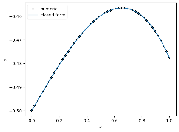
A plot of the above with a comparison to the exact expected values (obtained using the Airy functions of the first and second kind):