
Tutorial#
In this tutorial we will make the code we will write documentation for the code we wrote in the modularisation Tutorial.
There are a number of approaches to writing software documentation and I recommend reading the Further information.
We will start by creating a new file in VScode called README.md.
Attention
We will be writing our documentation in markdown.
Let us start by writing the title of our page and quick single sentence description.
# Absorption

Functionality to study the absorbing Markov chains.
Writing a tutorial#
We will then write our first section which is a tutorial.
Attention
The goal of a tutorial is to provide a hands on introduction and demonstration of the software.
## Tutorial

In this tutorial we will see how to use `absorption` to study an absorbing
Markov chain. For some background information on absorbing Markov chains we
recommend: <https://en.wikipedia.org/wiki/Absorbing_Markov_chain>.

Given a transition matrix $P$ defined by:

$$
p = \begin{pmatrix}
   1/2 & 1/4 & 1/4\\
   1/3 & 1/3 & 1/3\\
   0   & 0   & 1
    \end{pmatrix}
$$

We will start by seeing how the chain evolves over time by starting with an
initial vector $\pi=(1,0,0)$. In the next code snippet we will import the
necessary libraries and create both $P$ and $\pi$:

```python
import numpy as np

import absorption

pi = np.array([1, 0, 0])
P = np.array([[1 / 2, 1 / 4, 1 / 4], [1 / 3, 1 / 3, 1 / 3], [0, 0, 1]])
```

We now see how the vector $\pi$ changes over time:

```python
for k in range(10):
    print(absorption.get_long_run_state(pi, k, P))
```

This will give:

```
[1. 0. 0.]
[0.5  0.25 0.25]
[0.33333333 0.20833333 0.45833333]
[0.23611111 0.15277778 0.61111111]
[0.16898148 0.1099537  0.72106481]
[0.12114198 0.0788966  0.79996142]
[0.08686986 0.05658436 0.85654578]
[0.06229638 0.04057892 0.8971247 ]
[0.0446745 0.0291004 0.9262251]
[0.03203738 0.02086876 0.94709386]
```

We see that, as expected over time the probability of being in the third state,
which is absorbing, increases.

We can also use `absorption` to get the average number of steps until
absorption from each state:

```python
absorption.compute_t(P)
```

This gives:

```
array([3.66666667, 3.33333333])
```

We see that the expected amounts of steps from the first state is slightly more
than from the second.
This tutorial section allows newcomers to our code to see how it is intended to be used.
Writing the how-to guides#
In the next section we will write a series of how to guides, this is targeted at someone who has perhaps worked through the tutorial already and wants to directly know how to do a specific tasks.
Directly underneath what we have written so far we write:
## How to guides

### How to compute the long run state of a system after a given number of steps

Given a transition matrix $P$ and a state vector $\pi$, the state of the system
after $k$ steps is given by:

```python
import numpy as np

import absorption

pi = np.array([0, 1, 0])
P = np.array([[1 / 3, 1 / 3, 1 / 3], [1 / 4, 1 / 4, 1 / 2], [0, 0, 1]])
absorption.get_long_run_state(pi=pi, k=10, P=P)
```

This gives:

```
array([0.0019552, 0.0019552, 0.9960896])
```

### How to extract the transitive state transition sub matrix $Q$

Given a transition matrix $P$, the sub matrix $Q$ that
corresponds to the transitions between transitive (i.e. not absorbing) states can
be extracted:

```python
import numpy as np

import absorption

P = np.array([[1 / 3, 1 / 3, 1 / 3], [0, 1, 0], [1 / 4, 1 / 4, 1 / 2]])
absorption.extract_Q(P=P)
```

This gives:

```
array([[0.33333333, 0.33333333],
       [0.25      , 0.5       ]])
```

### How to compute the fundamental matrix $N$

Given a transition matrix $P$, the fundamental matrix $N$
can be obtained:

```python
import numpy as np

import absorption

P = np.array([[1 / 3, 1 / 3, 1 / 3], [0, 1, 0], [1 / 4, 1 / 4, 1 / 2]])
Q = absorption.extract_Q(P=P)
absorption.compute_N(Q=Q)
```

This gives:

```
array([[2.        , 1.33333333],
       [1.        , 2.66666667]])
```

### How to compute the average steps until absorption

Given a transition matrix $P$ and a state vector $\pi$, the average number of
steps until absorption from all states can be obtained:

```python
import numpy as np

import absorption

P = np.array([[1 / 3, 1 / 3, 1 / 3], [0, 1, 0], [1 / 4, 1 / 4, 1 / 2]])
absorption.compute_t(P=P)
```

This gives:

```
array([3.33333333, 3.66666667])
```
This how to section is an efficient collection of recipes to be able to carry out specific tasks made possible by the software.
Writing the explanations section#
In the next section we will write the explanations which aims to give more in depth understanding not necessarily directly related to the code.
## Explanation

### Brief overview of absorbing markov chains

A Markov chain with a given transition matrix $P$ is a system that moves from
state to state randomly with the probabilities given by $P$.

For example:

$$
P = \begin{pmatrix}
        1 / 3 & 1 / 3 & 1 / 3 \\
        0     & 1     & 0     \\
        1 / 4 & 1 / 4 & 1 / 2
    \end{pmatrix}
$$

The corresponding Markov chain has 3 states and:

- $P_{11}=1/3$ means that when in state 1 there is a 1/3 chance of staying in
  state 1.
- $P_{23}=0$ means that when in state 2 there is a 0 chance of staying in
  state 1.
- $P_{22}=$ actually implies that once we are in state 2 that the only next
  state is state 2.

In general:

$$
    P_{ij} > 0 \text{ for all }ij
$$

$$
    \sum_{j=0}^{|P|} P_{ij} = 1 \text{ for all }i
$$

If $P_{ii}=1$ then state $i$ is an absorbing state from which no further changes
can occur.

In the case of absorbing markov chains there are a number of quantities that can
be measured.

### Calculating the state after a given number of iterations

Given a vector that describes the state of the system $\pi$ and a transition
matrix $P$, the state of the system after $k$ iterations will be given by the
following vector:

$$
    \pi P ^ k
$$

### The canonical form of the transition matrix

A transition matrix $P$ is written in its canonical form when it can be written
as:

$$
  P =
  \left(\begin{array}{c|c}
    Q & R \\\hline
    0 & I
  \end{array}\right)
$$

Where $Q$ is the matrix of transitions between non absorbing states.

For example, the canonical form of $P$ would be:

$$
    \begin{pmatrix}
        1 / 3 & 1 / 3 & 1 / 3 \\
        1 / 4 & 1 / 2 & 1 / 4 \\
        0     &  0    & 1     \\
    \end{pmatrix}
$$

which would give:

$$
Q = \begin{pmatrix}
    1 / 3 & 1 / 3 \\
    1 / 4 & 1 / 2
    \end{pmatrix}
$$

### The fundamental matrix

Given $Q$ the fundamental matrix $N$ is defined as:

$$N = (I - Q) ^{-1}$$

$N_{ij}$ corresponds to the expected number of times the chain will be in state
$j$ given that it started in state $i$.

### The expected number of steps until absorption.

Given $N$, the expected number of steps until absorption is given by the vector:

$$
t = N \mathbb{1}
$$

where $\mathbb{1}$ denotes a vector of 1s.
This explanations section gives background reading as to how the code works.
Writing the reference section#
In the next section we will write the reference which aims to be a concise collection of reference material.
## Reference

### List of functionality

The following functions are written in `absorption`:

- `get_long_run_state`
- `extract_Q`
- `compute_N`
- `compute_t`

### Bibliography

The wikipedia page on absorbing Markov chains gives a good overview of the
topic: <https://en.wikipedia.org/wiki/Absorbing_Markov_chain>

The following text is a recommended reference on Markov chains:

> Stewart, William J. Probability, Markov chains, queues, and simulation: the
> mathematical basis of performance modelling. Princeton university press, 2009.
Figure The README.md file in VScode with the rendered preview (using the Markdown all in one plugin). shows the start of the markdown file
in VScode alongside the preview (the Markdown all in one plugin ensures that
the mathematics is rendered see Install VScode plugins for
information on installing plugins).
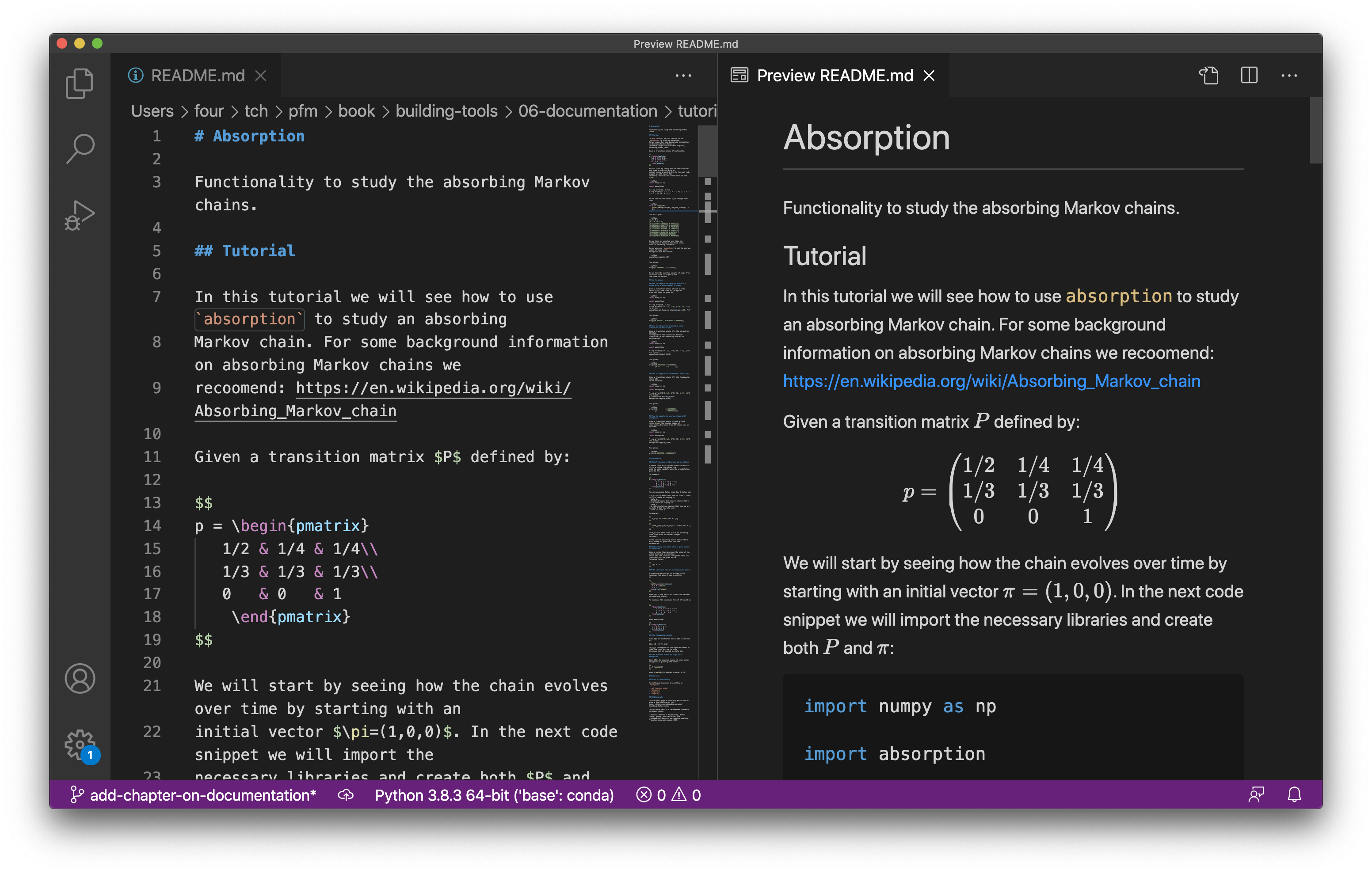
Fig. 34 The README.md file in VScode with the rendered preview (using the Markdown all in one plugin).#
Below is what the rendered documentation would look like:
Documentation for absorption#
Absorption#
Functionality to study the absorbing Markov chains.
Tutorial#
In this tutorial we will see how to use absorption to study an absorbing
Markov chain. For some background information on absorbing Markov chains we
recommend: https://en.wikipedia.org/wiki/Absorbing_Markov_chain.
Given a transition matrix \(P\) defined by:
We will start by seeing how the chain evolves over time by starting with an initial vector \(\pi=(1,0,0)\). In the next code snippet we will import the necessary libraries and create both \(P\) and \(\pi\):
import numpy as np

import absorption

pi = np.array([1, 0, 0])
P = np.array([[1 / 2, 1 / 4, 1 / 4], [1 / 3, 1 / 3, 1 / 3], [0, 0, 1]])
We now see how the vector \(\pi\) changes over time:
for k in range(10):
    print(absorption.get_long_run_state(pi, k, P))
This will give:
[1. 0. 0.]
[0.5  0.25 0.25]
[0.33333333 0.20833333 0.45833333]
[0.23611111 0.15277778 0.61111111]
[0.16898148 0.1099537  0.72106481]
[0.12114198 0.0788966  0.79996142]
[0.08686986 0.05658436 0.85654578]
[0.06229638 0.04057892 0.8971247 ]
[0.0446745 0.0291004 0.9262251]
[0.03203738 0.02086876 0.94709386]
We see that, as expected over time the probability of being in the third state, which is absorbing, increases.
We can also use absorption to get the average number of steps until
absorption from each state:
absorption.compute_t(P)
This gives:
array([3.66666667, 3.33333333])
We see that the expected amounts of steps from the first state is slightly more than from the second.
How to guides#
How to compute the long run state of a system after a given number of steps#
Given a transition matrix \(P\) and a state vector \(\pi\), the state of the system after \(k\) steps is given by:
import numpy as np

import absorption

pi = np.array([0, 1, 0])
P = np.array([[1 / 3, 1 / 3, 1 / 3], [1 / 4, 1 / 4, 1 / 2], [0, 0, 1]])
absorption.get_long_run_state(pi=pi, k=10, P=P)
This gives:
array([0.0019552, 0.0019552, 0.9960896])
How to extract the transitive state transition sub matrix \(Q\)#
Given a transition matrix \(P\), the sub matrix \(Q\) that corresponds to the transitions between transitive (i.e. not absorbing) states can be extracted:
import numpy as np

import absorption

P = np.array([[1 / 3, 1 / 3, 1 / 3], [0, 1, 0], [1 / 4, 1 / 4, 1 / 2]])
absorption.extract_Q(P=P)
This gives:
array([[0.33333333, 0.33333333],
       [0.25      , 0.5       ]])
How to compute the fundamental matrix \(N\)#
Given a transition matrix \(P\), the fundamental matrix \(N\) can be obtained:
import numpy as np

import absorption

P = np.array([[1 / 3, 1 / 3, 1 / 3], [0, 1, 0], [1 / 4, 1 / 4, 1 / 2]])
Q = absorption.extract_Q(P=P)
absorption.compute_N(Q=Q)
This gives:
array([[2.        , 1.33333333],
       [1.        , 2.66666667]])
How to compute the average steps until absorption#
Given a transition matrix \(P\) and a state vector \(\pi\), the average number of steps until absorption from all states can be obtained:
import numpy as np

import absorption

P = np.array([[1 / 3, 1 / 3, 1 / 3], [0, 1, 0], [1 / 4, 1 / 4, 1 / 2]])
absorption.compute_t(P=P)
This gives:
array([3.33333333, 3.66666667])
Explanation#
Brief overview of absorbing markov chains#
A Markov chain with a given transition matrix \(P\) is a system that moves from state to state randomly with the probabilities given by \(P\).
For example:
The corresponding Markov chain has 3 states and:
\(P_{11}=1/3\) means that when in state 1 there is a 1/3 chance of staying in state 1.
\(P_{23}=0\) means that when in state 2 there is a 0 chance of staying in state 1.
\(P_{22}=\) actually implies that once we are in state 2 that the only next state is state 2.
In general:
If \(P_{ii}=1\) then state \(i\) is an absorbing state from which no further changes can occur.
In the case of absorbing markov chains there are a number of quantities that can be measured.
Calculating the state after a given number of iterations#
Given a vector that describes the state of the system \(\pi\) and a transition matrix \(P\), the state of the system after \(k\) iterations will be given by the following vector:
The canonical form of the transition matrix#
A transition matrix \(P\) is written in its canonical form when it can be written as:
Where \(Q\) is the matrix of transitions between non absorbing states.
For example, the canonical form of \(P\) would be:
which would give:
The fundamental matrix#
Given \(Q\) the fundamental matrix \(N\) is defined as:
\(N_{ij}\) corresponds to the expected number of times the chain will be in state \(j\) given that it started in state \(i\).
The expected number of steps until absorption.#
Given \(N\), the expected number of steps until absorption is given by the vector:
where \(\mathbb{1}\) denotes a vector of 1s.
Reference#
List of functionality#
The following functions are written in absorption:
get_long_run_stateextract_Qcompute_Ncompute_t
Bibliography#
The wikipedia page on absorbing Markov chains gives a good overview of the topic: https://en.wikipedia.org/wiki/Absorbing_Markov_chain
The following text is a recommended reference on Markov chains:
Stewart, William J. Probability, Markov chains, queues, and simulation: the mathematical basis of performance modelling. Princeton university press, 2009.