Tutorial

We will here consider a problem we have already solved (in the Algebra Tutorial) but use a different interface to do so than Jupyter. The code itself will be the same. The way we run it will differ.

Problem

Rationalise the denominator of \(\frac{1}{\sqrt{2} + 1}\)

Open a command line tool:

1. On Windows search for Anaconda Prompt (it should be available to you after installing Anaconda). See Starting the notebook server on Windows.

2. On OS X search for terminal. See Starting the notebook server on MacOS.

Whether or not your are on Windows or MacOS changes the commands you need to type. We will first list the directory we are currently in:

Windows

$ dir

MacOS

$ ls

Tip

Throughout this book, when there are commands to be typed in a command line tool I will prefix them with a $. Do not type the $.

This is similar to using your file explorer to view the contents in a given directory. Similarly to the way we click on a directory in the file explorer we can navigate to a directory in the command line.

To do this we use the same command on both operating systems:

Windows

$ cd <target_directory_name>

MacOS

$ cd <target_directory_name>

We will do this to navigate to our cfm directoy. For example if, as in the Algebra Tutorial the cfm directory was on the Desktop directory we would run the following:

Windows

$ cd Desktop
$ cd cfm

MacOS

$ cd Desktop
$ cd cfm

Attention

The two statements are written under each other to denote that they are run one after the other.

We will now create a new directory:

Windows

$ mkdir scripts

MacOS

$ mkdir scripts

Inside this directory we will run the same command as before to see the contents:

Windows

$ dir

MacOS

$ ls

If you have followed the same steps described in Using notebooks then you will see something similar to:

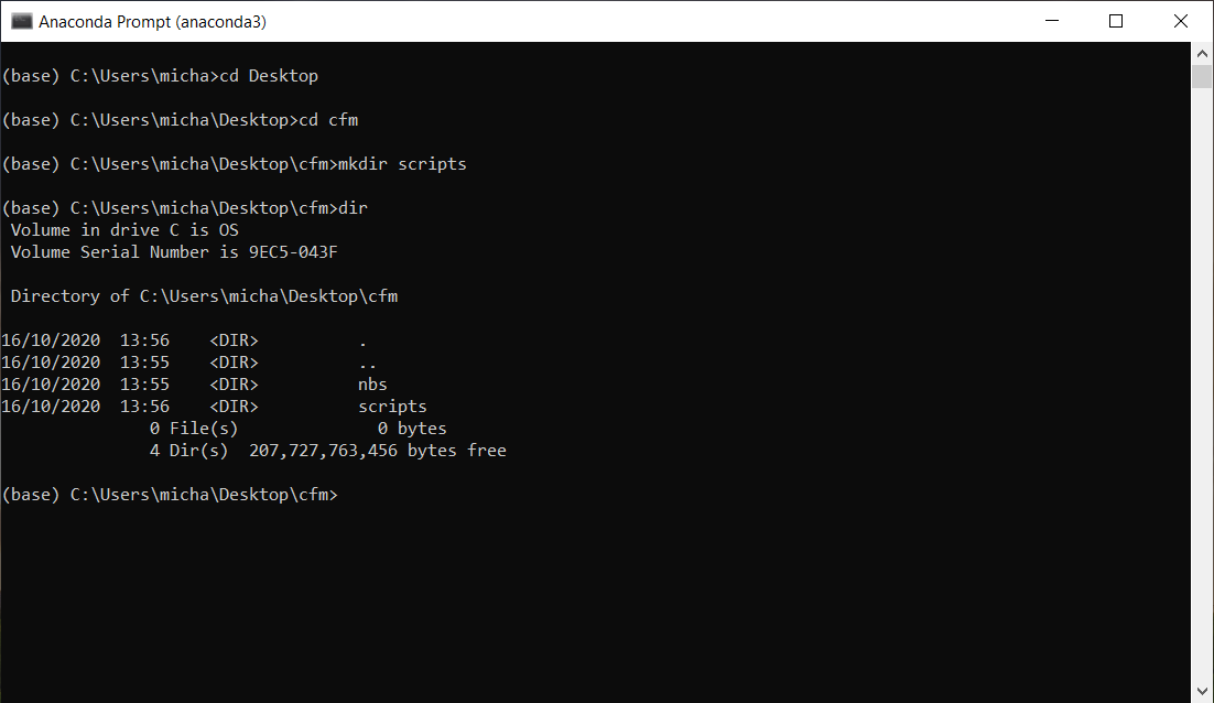
Fig. 12 The contents of our directory on Windows

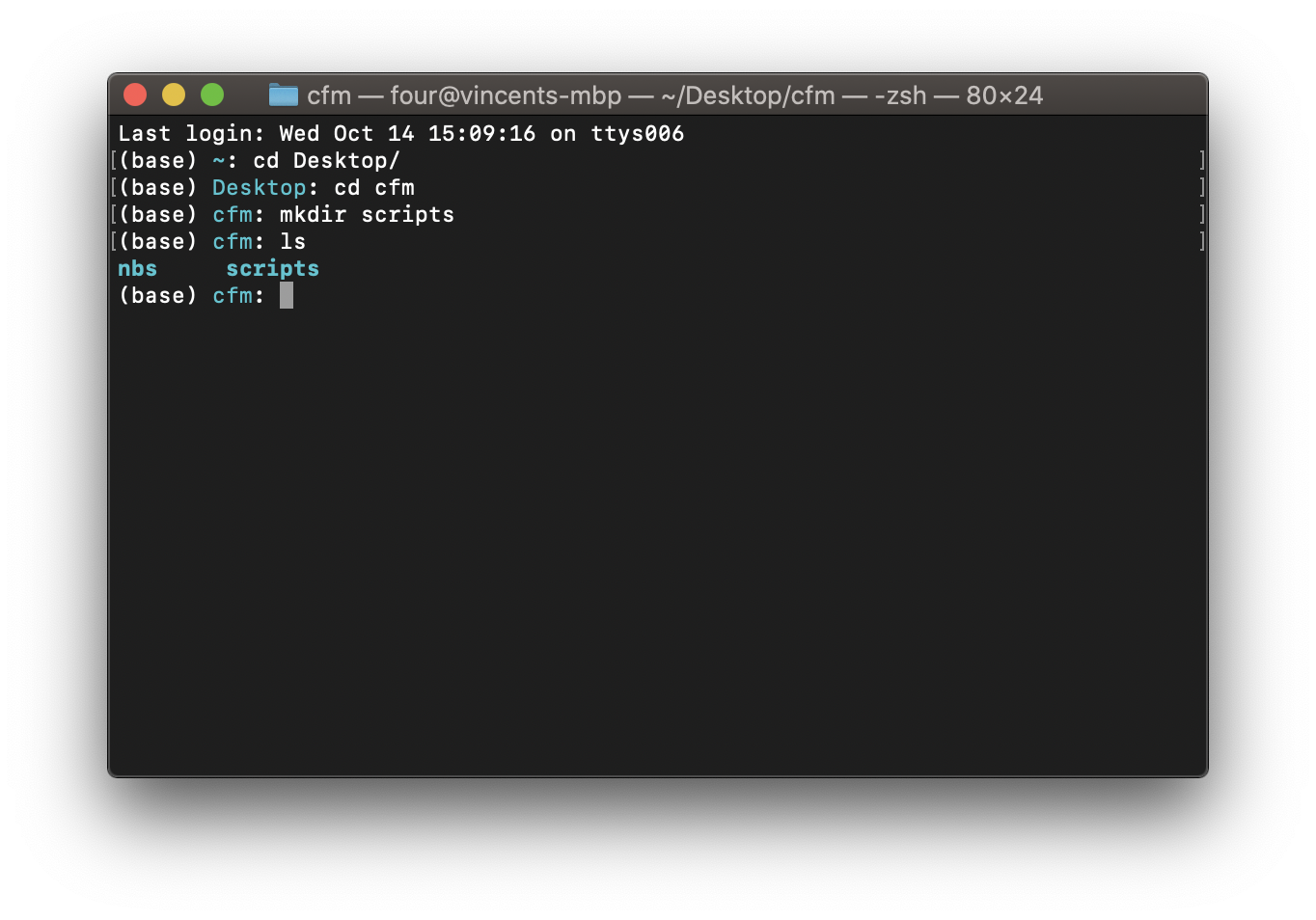
Fig. 13 The contents of our directory on OS X

We will come back to this directory shortly but now we are going to install a powerful code editor.

1. Navigate to https://code.visualstudio.com.

2. Download the installer making sure it is the correct one for your operating system (Windows, Mac OSX, Linux).

3. Run the installer.

This code editor will offer us a different way to write Python code.

Open VS code and create a new file.

In it write the following (which corresponds to the solution of our problem):

"""
This script displays the solution to the problem considered.
"""
import sympy as sym

print("Question 1:")
expression = 1 / (sym.sqrt(2) + 1)
print(sym.simplify(expression))

This is shown:

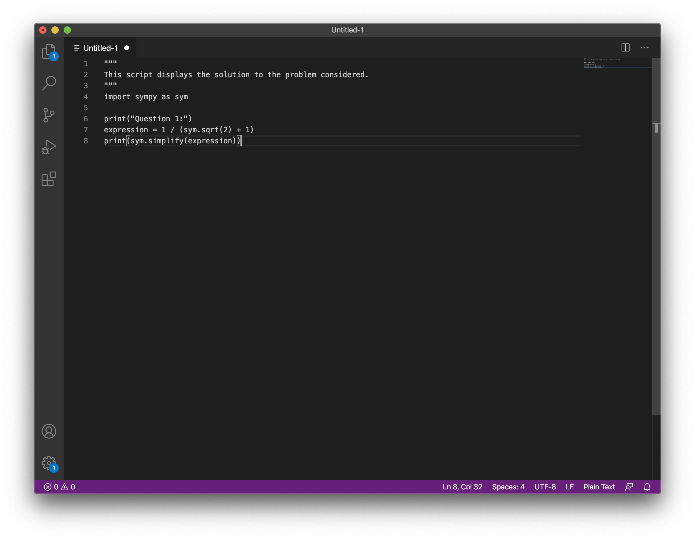
Fig. 14 The code above in VS code

We will now save this as algebra.py inside the scripts directory we created earlier.

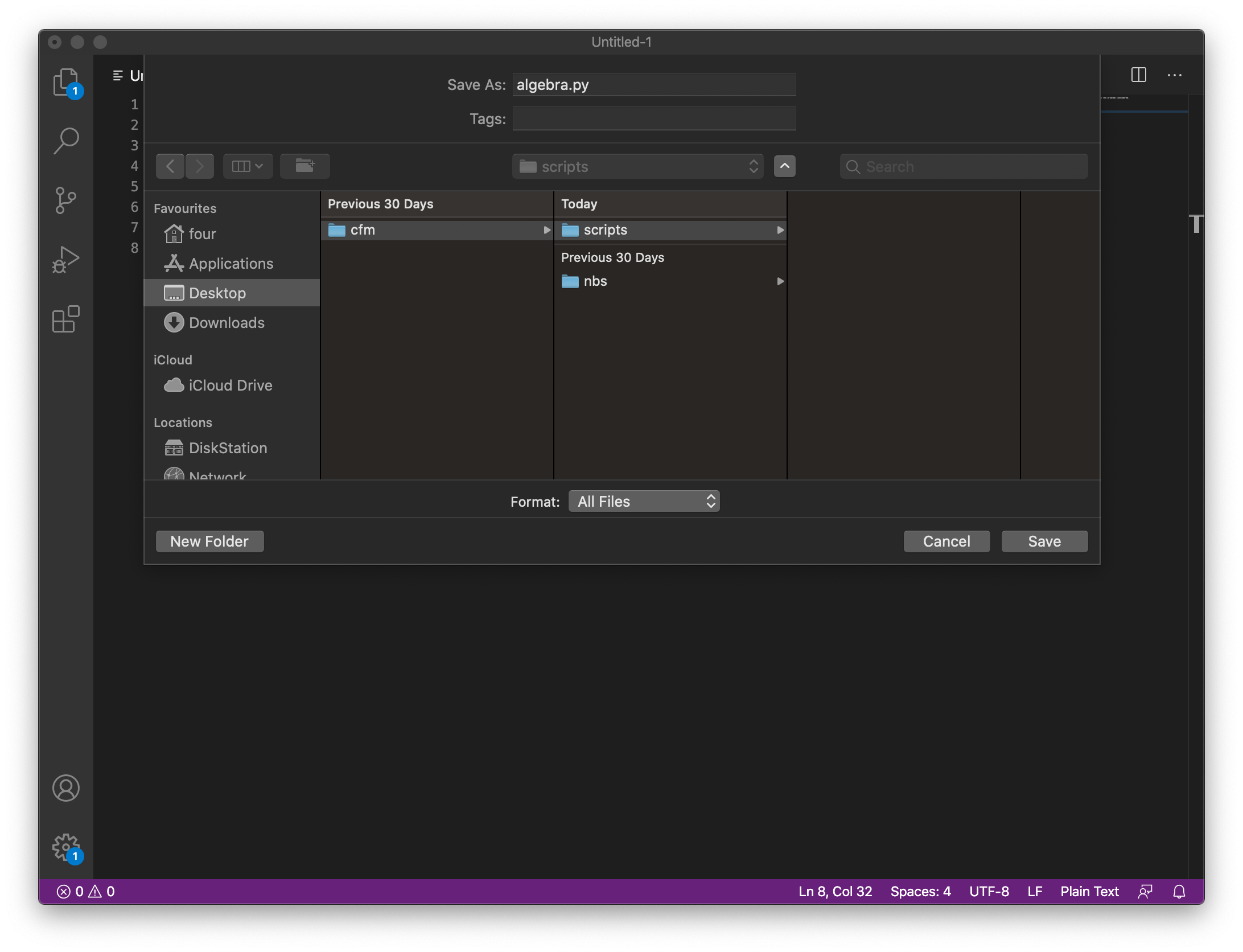
Fig. 15 Saving algebra.py in VS code.

VScode now recognises the Python language and adds syntax colouring. It also suggests a plugin specific for the Python language. There is more information about plugins in the rest of this chapter.

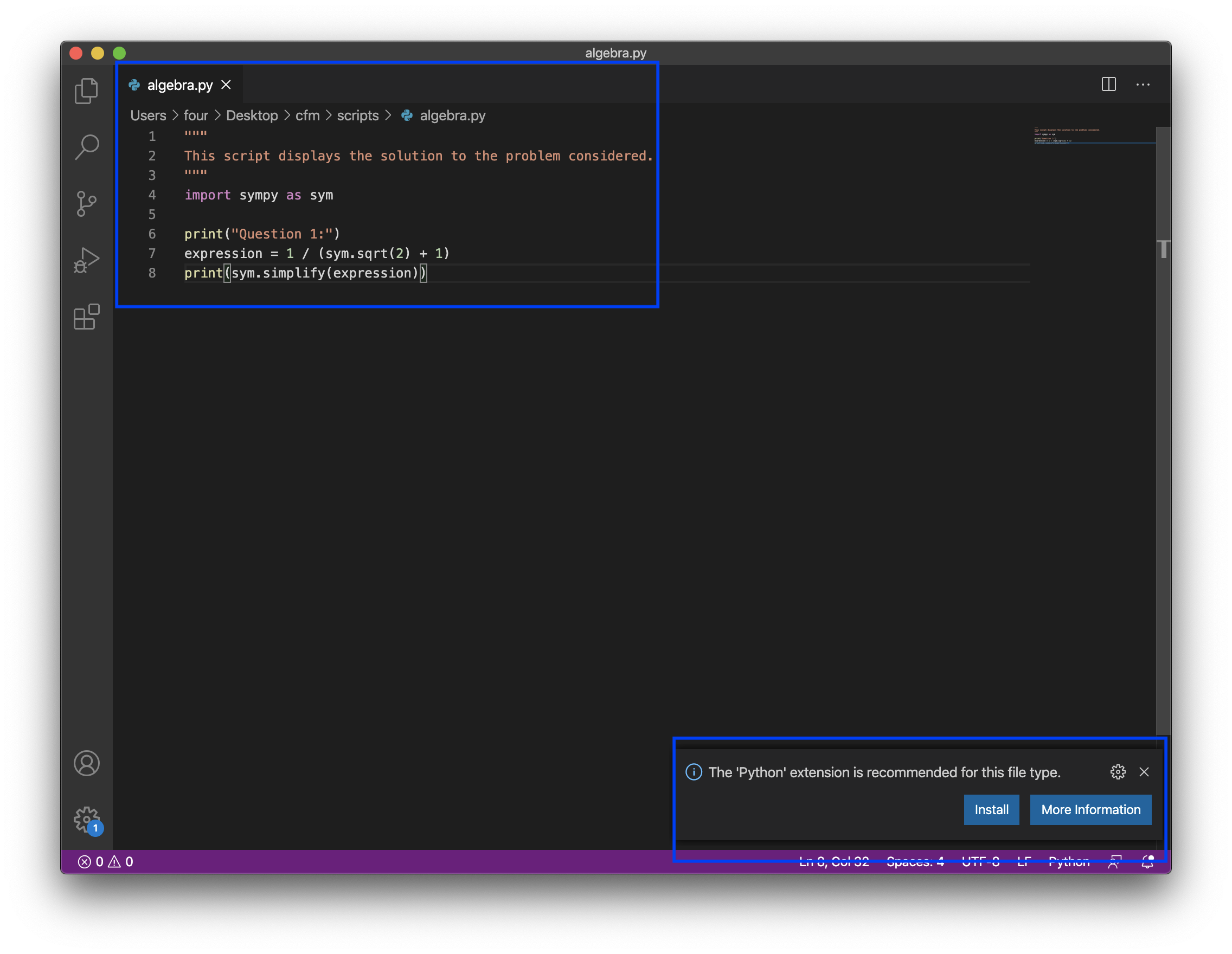
Fig. 16 Syntax colouring and plugin suggestion for the now recognised Python file.

All we have done so far is write the code. We now need to tell Python to run it. To do this we will use the command line.

Navigate to the scripts directory that we created earlier:

Windows

$ cd scripts

MacOS

$ cd scripts

Now confirm that the algebra.py file is in that directory:

Windows

$ dir

MacOS

$ ls

Now we will run the python code in that script:

$ python algebra.py

When doing that you should see the following output:

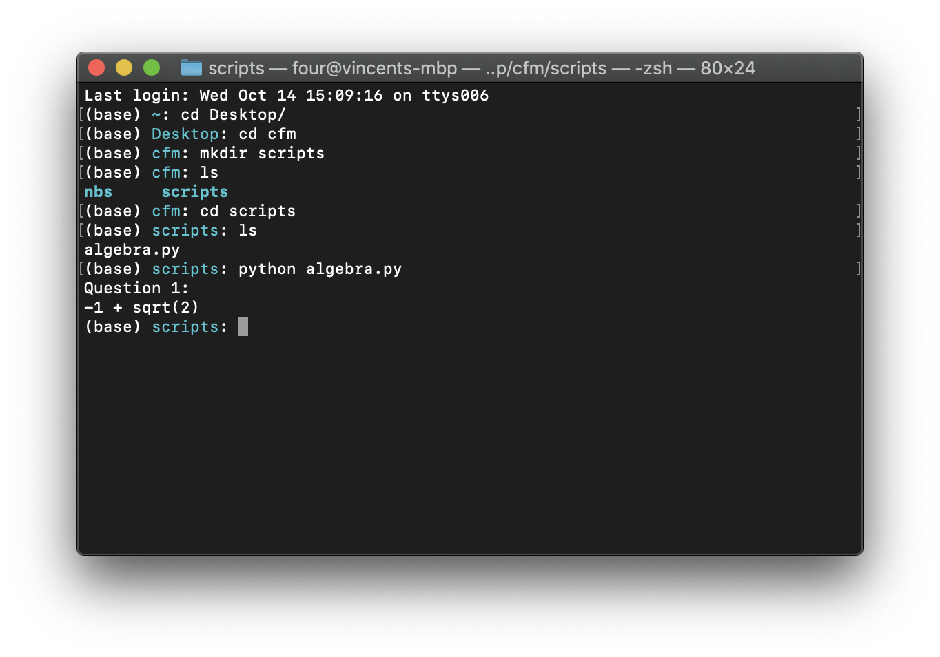
Fig. 17 Output of running the algebra.py script on OS X.