
Tutorial#
You will solve the following problem using a computer to do some of the more tedious calculations.
Problem
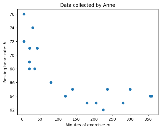
Anna is investigating the relationship between exercise and resting heart rate. She takes a of 19 people in her year group and records for each person
their resting heart rate, \(h\) beats per minute.
the number of minutes, \(m\), spent exercising each week.
A table with the data is here:
h |
m |
|---|---|
76.0 |
5 |
72.0 |
5 |
71.0 |
21 |
74.0 |
30 |
71.0 |
42 |
69.0 |
20 |
68.0 |
20 |
68.0 |
35 |
66 |
80.0 |
64 |
120.0 |
65 |
140.0 |
63 |
180.0 |
63 |
205.0 |
62 |
225.0 |
65 |
237.0 |
63 |
280.0 |
65 |
300.0 |
64 |
356.0 |
64 |
360.0 |
You can see a scatter plot below.
For all collected values of \(h\) and \(m\) obtain:
The mean
The median
The quartiles
The standard deviation
The variation
The maximum
The minimum
Obtain the Pearson Coefficient of correlation for the variables \(h\) and \(m\).
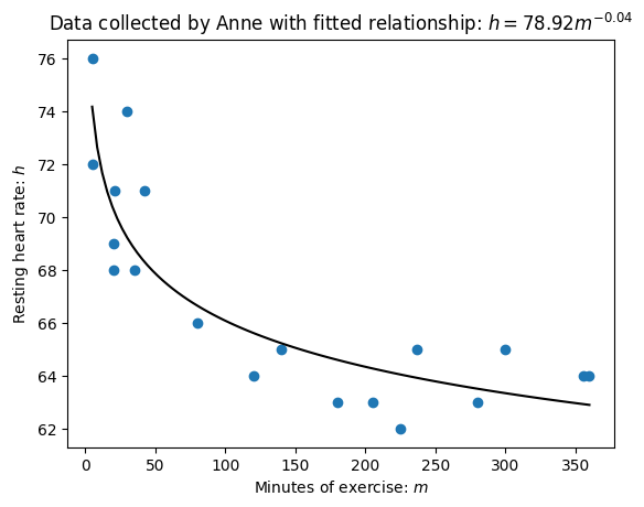
Obtain the line of best fit for variables \(x\) and \(y\) as defined by: $\(\begin{split}x=\ln(m)\qquad y=\ln(h)\end{split}\)$
Using the above obtain a relationship between \(m\) and \(h\) of the form: $\(\begin{split}h=cm^k\end{split}\)$
Start by inputting all the data:
h = (
    76.0,
    72.0,
    71.0,
    74.0,
    71.0,
    69.0,
    68.0,
    68.0,
    66.0,
    64.0,
    65.0,
    63.0,
    63.0,
    62.0,
    65.0,
    63.0,
    65.0,
    64.0,
    64.0,
)
m = (
    5,
    5,
    21,
    30,
    42,
    20,
    20,
    35,
    80,
    120,
    140,
    180,
    205,
    225,
    237,
    280,
    300,
    356,
    360,
)
The main tool you are going to use for this is statistics.
import statistics as st
To calculate the mean:
st.mean(h)
67.0
st.mean(m)
140.05263157894737
To calculate the median:
st.median(h)
65.0
st.median(m)
120
To calculate the quartiles, use statistics.quantiles and specify that you
want to separate the date into \(n=4\) quarters.
st.quantiles(h, n=4)
[64.0, 65.0, 71.0]
st.quantiles(m, n=4)
[21.0, 120.0, 237.0]
Note that this calculation confirms the median which corresponds to the 50% quartile. To calculate the sample standard deviation:
st.stdev(h)
4.123105625617661
st.stdev(m)
124.46662813970593
To calculate the sample variance:
st.variance(h)
17.0
st.variance(m)
15491.941520467837
To compute that maximum:
max(h)
76.0
max(m)
360
To compute the minimum:
min(h)
62.0
min(m)
5
In order to compute the Pearson Coefficient of correlation use
statistics.correlation:
st.correlation(h, m)
-0.7686142969026402
This negative value indicates a negative correlation between \(h\) and \(m\), indicating that the more you exercise the lower your heart rate is likely to be.
To calculate the line of best fit for the transformed variables we need to first
create them. We will do this using a list comprehension. As you are doing
everything numerically, we will use math.log which by default computes the
natural logarithm:
import math
x = [math.log(value) for value in m]
y = [math.log(value) for value in h]
Now to compute the line of best fit use statistics.linear_regression:
slope, intercept = st.linear_regression(x, y)
The slope is:
slope
-0.03854770754231997
The intercept is:
intercept
4.368415819445762
Recall the transformation of the variables:
You now have the relationship:
Where \(a\) corresponds to the slope and \(b\) corresponds to the intercept.
The question asks for a relationship between \(m\) and \(h\) of the form:
You can use sympy to manipulate the expressions:
import sympy as sym

h = sym.Symbol("h")
m = sym.Symbol("m")
a = sym.Symbol("a")
b = sym.Symbol("b")
x = sym.ln(m)
y = sym.ln(h)
A general line of best fit for \(x\) and \(y\) can be expressed in terms of \(m\) and \(h\):
line = sym.Eq(lhs=y, rhs=a * x + b)
line
Taking the exponential of both sides gives the required relationship:
sym.exp(line.lhs)
sym.expand(sym.exp(line.rhs))
Which can be rewritten as:
Substituting our values for the slope and intercept into these expressions
gives the required relationship:
sym.exp(line.rhs).subs({a: slope, b: intercept})
Below is a plot that shows this relationship:
Important
In this tutorial you have
Calulated values of central tendency and spread;
Calculated some bivariate coefficient;
Fitted a line of best fit.