Motivating Example: Construction Contractors
Consider two local construction firms, Firm A and Firm B, who regularly bid on municipal infrastructure projects.
Each quarter, the city may announce a new contract for firms to bid on — a school, a road, or a public facility. These firms can choose to:
Bid High (H): maintain high prices and sustain mutual profitability, or
Bid Low (L): undercut the other firm to win the project outright.
If both firms bid high, they enjoy good margins and may take turns winning contracts. If one undercuts while the other bids high, the undercutter wins the project and earns a higher profit, at the cost of undermining trust. If both bid low, a price war ensues, shrinking profits for both.
However, the number of projects is not fixed in advance. After each bidding round, there is a probability that another project becomes available. Thus, the game is repeated probabilistically, with continuation probability . The expected number of repetitions is .
Each firm chooses an action in each round:
: Bid High
: Bid Low
The one-shot payoff matrix is given by:
This is a classic example of a Prisoner’s Dilemma: short-term incentives tempt each player to defect (bid low), but long-term cooperation (bid high) could yield better payoffs.
The remainder of this chapter will explore:
How cooperation can be sustained using history-dependent strategies.
What conditions on allow for equilibrium cooperation.
The formal statement and implications of the Folk Theorem.
The concept of direct reciprocity.
Theory
Definition: repeated game
Given a two player game , referred to as a stage game, a -stage repeated game is a game in which players play that stage game for repetitions. Players make decisions based on the full history of play over all the repetitions.
Example: Counting leaves in repeated games
Consider the following stage games and values of . How many leaves would the extensive form representation of the repeated game have?
The initial play of the game has 4 outcomes (2 actions each). Each of these leads to 4 more in the second stage. Total: leaves.
Same as (1): leaves.
Three stages of 2 actions each: leaves.
First stage: outcomes. Each of those leads to 6 in the second stage. Total: leaves.
Definition: Strategies in a repeated game
A strategy for a player in a repeated game is a mapping from all possible histories of play to a probability distribution over the action set of the stage game.
Example: Validity of repeated game strategies
For the Coordination Game with determine whether the following strategy pairs are valid, and if so, what outcome they lead to.
Row player:
Column player:
Valid strategy pair. Outcome: (corresponds to in the extensive form).
Row player:
Column player:
Invalid: the row player does not define an action for history .
Row player:
Column player:
Invalid: column player uses an invalid action .
Row player:
Column player:
Valid strategy pair. Outcome: (corresponds to in the extensive form).
Theorem: Subgame perfection of sequence of stage Nash profiles
For any repeated game, any sequence of stage Nash profiles gives the outcome of a subgame perfect Nash equilibrium.
Where by stage Nash profile we refer to a strategy profile that is a Nash Equilibrium in the stage game.
Proof
If we consider the strategy given by:
“Player should play strategy regardless of the play of any previous strategy profiles.”
where is the strategy played by player in any stage Nash profile. The is used to indicate that all players play strategies from the same stage Nash profile.
Using backwards induction we see that this strategy is a Nash equilibrium. Furthermore it is a stage Nash profile so it is a Nash equilibria for the last stage game which is the last subgame. If we consider (in an inductive way) each subsequent subgame the result holds.
Example
Consider the following stage game:
There are two Nash equilibria in action space for this stage game:
For we have 4 possible outcomes that correspond to the outcome of a subgame perfect Nash equilibria:
Importantly, not all subgame Nash equilibria outcomes are of the above form.
Reputation
In a repeated game it is possible for players to encode reputation and trust in their strategies.
Example: Reputation in a repeated game
Consider the following stage game with :
Through inspection it is possible to verify that the following strategy pair is a Nash equilibrium.
For the row player:
For the column player:
This pair of strategies corresponds to the following scenario:
The row player plays and the column player plays in the first stage. The row player plays and the column player plays in the second stage.
Note that if the row player deviates and plays in the first stage, then the column player will play in the second stage.
If both players play these strategies, their utilities are: , which is better for both players than the utilities at any sequence of stage Nash equilibria in action space.
But is this a Nash equilibrium? To find out, we investigate whether either player has an incentive to deviate.
If the row player deviates, they would only be rational to do so in the first stage. If they did, they would gain 1 in that stage but lose 4 in the second stage. Thus they have no incentive to deviate.
If the column player deviates, they would only do so in the first stage and gain no utility.
Thus, this strategy pair is a Nash equilibrium and evidences how reputation can be built and cooperation can emerge from complex dynamics.
Definition: Infinitely Repeated Game with Discounting
Given a two player game , referred to as a stage game, an infinitely repeated game with discounting factor is a game in which players play that stage game an infinite amount of times and gain the following utility:
where denotes the utility obtained in the stage game for actions and which are the actions given by strategies and at stage .
Example:
Consider Motivating Example: Construction Contractors and assume Firm A plans to undercut at all contracts: bidding low. Firm B plans to start by cooperating (bidding high) but if Firm A ever undercuts then Firm B will undercut for all subsequent contracts.
and
Replacing the values from the stage game this gives:
Definition: Average utility
If we interpret as the probability of the repeated game not ending then the average length of the game is:
We can use this to define the average payoff per stage:
Example:
Consider 3 strategies for Motivating Example: Construction Contractors:
Always cooperate: bid high on all contracts.
Always defect: bid low on all contracts.
Grudger: bid high until facing a low bid and then bid low for ever.
For :
Obtain the 3 by 3 Normal form game using average utility.
Check if mutual cooperation is a Nash equilibrium for both games.
We construct the Normal Form game representation with the 3 strategies becoming the action space (as described in Mapping Extensive Form Games to Normal Form).
We see that if is played against then both players cooperate at each stage giving:
For and we have:
For and we repeat the calculations of Example: to obtain:
and
Using the action space ordered as: this gives:
The game is symmetric so:
For this gives:
The game is symmetric so:
We see that and are both dominated by thus mutual cooperation is not a Nash equilibrium.
For this gives:
The game is symmetric so:
We see that mutual cooperation now is a Nash equilibrium because is now a best response to .
The fact that cooperation can be stable for a higher value of is in fact a theorem that holds in the general case.
We need one final definition to describe what we imply:
Definition of individually rational payoffs
Individually rational payoffs are average payoffs that exceed the stage game Nash equilibrium payoffs for both players.
As an example consider the plot corresponding to a repeated Prisoner’s Dilemma shown in Figure 1.
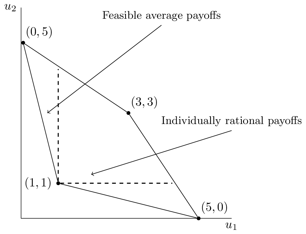
Figure 1:The convex hull of payoffs for the Prisoner’s Dilemma.
The feasible average payoffs correspond to the feasible payoffs in the stage game. The individually rational payoffs show the payoffs that are better for both players than the stage Nash equilibrium.
The following theorem states that we can choose a particular discount rate that for which there exists a subgame perfect Nash equilibrium that would give any individually rational payoff pair!
Theorem: Folk Theorem
Let be a pair of Nash equilibrium payoffs for a stage game. For every individually rational pair there exists such that for all there is a subgame perfect Nash equilibrium with payoffs .
Proof
Let be the stage Nash profile that yields . Now assume that playing and in every stage gives (an individual rational payoff pair).
Consider the following strategy:
“Begin by using and continue to use as long as both players use the agreed strategies. If any player deviates: use for all future stages.”
We begin by proving that the above is a Nash equilibrium.
Without loss of generality if player 1 deviates to such that in stage then:
Recalling that player 1 would receive in every stage with no deviation, the biggest gain to be made from deviating is if player 1 deviates in the first stage (all future gains are more heavily discounted). Thus if we can find such that implies that then player 1 has no incentive to deviate.
as , taking gives the required required result for player 1 and repeating the argument for player 2 completes the proof of the fact that the prescribed strategy is a Nash equilibrium.
By construction this strategy is also a subgame perfect Nash equilibrium. Given any history both players will act in the same way and no player will have an incentive to deviate:
If we consider a subgame just after any player has deviated from then both players use .
If we consider a subgame just after no player has deviated from then both players continue to use .
Definition: Prisoner’s Dilemma
The general form is:
with the following constraints:
The first constraint ensures that the second action “Defect” dominates the first action “Cooperate”.
The second constraint ensures that a social dilemma arises: the sum of the utilities to both players is best when they both cooperate.
This game is a good model of agent (human, etc) interaction: a player can choose to take a slight loss of utility for the benefit of the other player and themselves.
Example: Simplifed form of the Prisoner’s Dilemma:
Under what conditions is the following game a Prisoner’s Dilemma:
This is a Prisoner’s Dilemma when:
and:
Both of these equations hold for , in fact the second equation holds for all . This is a convenient form for the Prisoner’s Dilemma as it corresponds to a 1-dimensional parametrization.
As a single one-shot game there is not much more to say about the Prisoner’s Dilemma. It becomes fascinating when studied as a repeated game.
Axelrod’s tournaments
In 1980, political scientist Robert Axelrod organized a computer tournament for an iterated Prisoner’s Dilemma, as described in Axelrod, 1980.
Fourteen strategies were submitted.
The tournament was a round-robin of 200 iterations, including a fifteenth player who played uniformly at random.
Some submissions were highly sophisticated—for example, one strategy used a test to detect opponents behaving randomly. Further details can be found here.
The winner (by average score) was a surprisingly simple strategy: Tit For Tat, which begins by cooperating and then mimics the opponent’s previous move.
Following this, Axelrod hosted a second tournament with 62 strategy submissions Axelrod, 1980, again including a random strategy. Participants in this second round were aware of the original results, and many strategies were designed specifically to counter or improve upon Tit For Tat. Nonetheless, Tit For Tat prevailed once again.
These tournaments led to the wide acceptance of four principles for effective cooperation:
Do not be envious: avoid striving for a higher payoff than your opponent.
Be nice: never be the first to defect.
Reciprocate: respond to cooperation with cooperation, and to defection with defection.
Avoid overcomplication: do not attempt to outwit or exploit the opponent with excessive cunning.
These early experiments with the repeated Prisoner’s Dilemma were not only influential in political science but also laid a foundation for the study of emergent cooperation in multi-agent systems.
Exercises
Programming
Using Nashpy to generate repeated games
The Nashpy library has support for generating repeated games. Let us generate the repeated game obtained from the Prisoners Dilemma with :
import nashpy.repeated_games

import nashpy as nash
import numpy as np

M_r = np.array([[3, 0], [5, 1]])
M_c = M_r.T
prisoners_dilemma = nash.Game(M_r, M_c)
repeated_pd = nash.repeated_games.obtain_repeated_game(game=prisoners_dilemma, repetitions=2)
repeated_pd
Bi matrix game with payoff matrices:
Row player:
[[ 6. 6. 6. ... 3. 0. 0.]
[ 6. 6. 6. ... 3. 0. 0.]
[ 6. 6. 6. ... 3. 0. 0.]
...
[ 8. 8. 8. ... 2. 6. 2.]
[10. 10. 10. ... 1. 4. 1.]
[10. 10. 10. ... 2. 6. 2.]]
Column player:
[[ 6. 6. 6. ... 8. 10. 10.]
[ 6. 6. 6. ... 8. 10. 10.]
[ 6. 6. 6. ... 8. 10. 10.]
...
[ 3. 3. 3. ... 2. 1. 2.]
[ 0. 0. 0. ... 6. 4. 6.]
[ 0. 0. 0. ... 2. 1. 2.]]We can directly obtain the action space of the row player for a given repeated game as a python generator:
strategies = nash.repeated_games.obtain_strategy_space(A=M_r, repetitions=2)
len(list(strategies))32To obtain the action space for the columbn player use A=M_c.T:
strategies = nash.repeated_games.obtain_strategy_space(A=M_c.T, repetitions=2)
len(list(strategies))32Using the Axelrod library to study the repeated Prisoners Dilemma
There is a python library called axelrod which has functionality to run
tournaments akin to Robert Axelrod’s original tournaments but also includes
more than 240 total strategies as well as further functionality.
To generate a tournament with 4 strategies with
Tit For Tat: starts by cooperating, then repeats the opponent’s previous action.
Alternator: starts by cooperating, then alternates between cooperation and defection.
75% cooperator: a random strategy that cooperates 75% of the time.
Grudger: starts by cooperating, then defects forever if the opponent ever defects against it.
First let us set up some parameters such as the players as well as the seed to ensure reproducibility of the random results.
import axelrod as axl

players = [axl.TitForTat(), axl.Alternator(), axl.Random(.75), axl.Grudger()]
delta = 1 / 4
seed = 0
repetitions = 500
prob_end = 1 - delta
Now we create and run the tournament obtaining the payoff matrix from the results:
tournament = axl.Tournament(players=players, prob_end=prob_end, seed=seed, repetitions=repetitions)
results = tournament.play(progress_bar=False)
M_r = np.array(results.payoff_matrix)
M_r
array([[3. , 2.65566667, 2.30993333, 3. ],
[3.19483333, 2.74095238, 2.50883333, 3.17229048],
[3.39243333, 3.091 , 2.68228333, 3.38186667],
[3. , 2.67714762, 2.31336667, 3. ]])Notable research
The most influential early research on repeated games comes from the two seminal papers by Robert Axelrod Axelrod, 1980Axelrod, 1980, which culminated in his widely cited book Axelrod, 1984. As discussed in Section 6, Axelrod’s findings included a set of heuristics for successful behavior in the repeated Prisoner’s Dilemma.
Subsequent work has challenged these principles. The development of the Axelrod Python library Knight et al., 2016 enabled systematic and reproducible analysis across a far greater population of strategies. In particular, Glynatsi et al., 2024 studied 45,600 tournaments across diverse strategic populations and parameter regimes, finding that the original heuristics do not generalize. The revised empirical findings suggest the following properties are associated with successful play:
Be a little bit envious.
Be “nice” in non-noisy environments or when game lengths are longer.
Reciprocate both cooperation and defection appropriately; be provocable in tournaments with short matches and generous in noisy environments.
It is acceptable to be clever.
Adapt to the environment; adjust to the mean population cooperation rate.
The observation that being envious can be beneficial echoes a more recent development that was famously described by MIT Technology Review as having set “the world of game theory on fire”. In their landmark paper, Press & Dyson, 2012 introduced a novel class of memory-one strategies called zero-determinant strategies, which can unilaterally enforce linear payoff relationships, including extortionate dynamics.
However, the excitement around these strategies has been tempered by further theoretical and computational research. Studies such as Hilbe et al., 2013Knight et al., 2018 demonstrate that extortionate strategies, while elegant, do not tend to survive under evolutionary dynamics. These results reinforce the importance of adaptability and contextual behavior in long-run strategic success.
The Folk Theorem presented in this chapter can be traced to foundational work by Friedman, 1971 (with a correction in Friedman, 1973) and the general formulation in Fudenberg & Maskin, 1986. These theoretical insights laid the groundwork for subsequent developments such as Young, 1993, which shows how social conventions and norms can emerge from adaptive play in repeated settings.
Conclusion
Repeated games introduce a rich strategic landscape where history matters and reputation can sustain cooperation. Unlike one-shot interactions, repeated games allow for long-term incentives to shape behavior, often leading to outcomes that dominate those of stage game equilibria.
This chapter explored key ideas including the formal definitions of repeated and infinitely repeated games, strategy spaces based on full histories, subgame perfection through sequences of Nash profiles, and the pivotal role of discounting. Through examples and the Folk Theorem, we saw how cooperation can emerge—even in environments like the Prisoner’s Dilemma—when players value the future sufficiently.
In addition to theoretical foundations, we examined computational tools such as the Nashpy and Axelrod libraries, which allow for large-scale simulations and reproducible research into emergent cooperative behavior. We also revisited classical findings, including Axelrod’s tournaments, and contrasted them with modern insights that challenge early heuristics. A summary of key concepts is given in Table 1.
Table 1:The main linear programs for Zero Sum Game
| Concept | Description |
|---|---|
| Repeated game | A game consisting of multiple repetitions of a fixed stage game |
| Strategy in repeated game | A mapping from history of play to actions |
| Subgame perfect equilibrium | An equilibrium where players play a Nash profile in every subgame |
| Reputation | Players may cooperate to sustain credibility and trust over time |
| Discount factor () | Models time preference or probability of continuation |
| Average utility | Weighted utility that accounts for as average continuation length |
| Folk Theorem | Any individually rational payoff can be sustained given is high enough |
| Prisoner’s Dilemma | A canonical stage game often used to model cooperation and defection |
| Zero-determinant strategies | Memory-one strategies capable of extorting opponents (not evolutionarily stable) |
| Axelrod’s tournaments | Early empirical work showing Tit for Tat’s success in repeated dilemmas |
- Axelrod, R. (1980). Effective choice in the prisoner’s dilemma. Journal of Conflict Resolution, 24(1), 3–25.
- Axelrod, R. (1980). More effective choice in the prisoner’s dilemma. Journal of Conflict Resolution, 24(3), 379–403.
- Axelrod, R. (1984). The Evolution of Cooperation. Basic Books.
- Knight, V. A., Campbell, O., Harper, M., Langner, K. M., Campbell, J., Campbell, T., Carney, A., Chorley, M., Davidson-Pilon, C., Glass, K., & others. (2016). An open framework for the reproducible study of the iterated prisoner’s dilemma. Journal of Open Research Software, 4(1).
- Glynatsi, N. E., Knight, V., & Harper, M. (2024). Properties of winning Iterated Prisoner’s Dilemma strategies. PLOS Computational Biology, 20(12), e1012644.
- Press, W. H., & Dyson, F. J. (2012). Iterated Prisoner’s Dilemma contains strategies that dominate any evolutionary opponent. Proceedings of the National Academy of Sciences, 109(26), 10409–10413.
- Hilbe, C., Nowak, M. A., & Sigmund, K. (2013). Evolution of extortion in iterated prisoner’s dilemma games. Proceedings of the National Academy of Sciences, 110(17), 6913–6918.
- Knight, V., Harper, M., Glynatsi, N. E., & Campbell, O. (2018). Evolution reinforces cooperation with the emergence of self-recognition mechanisms: An empirical study of strategies in the Moran process for the iterated prisoner’s dilemma. PloS One, 13(10), e0204981.
- Friedman, J. W. (1971). A non-cooperative equilibrium for supergames. The Review of Economic Studies, 38(1), 1–12.
- Friedman, J. W. (1973). A non-cooperative equilibrium for supergames: A correction. The Review of Economic Studies, 40(3), 435–435.
- Fudenberg, D., & Maskin, E. (1986). The folk theorem in repeated games with discounting or with incomplete information. Econometrica, 54(3), 533–554.
- Young, H. P. (1993). The evolution of conventions. Econometrica: Journal of the Econometric Society, 57–84.