Motivating Example
Consider the following scenario: you would like to meet your friends for coffee. You know the following about their behavior:
With probability 20%, they choose coffee house A.
With probability 80%, they choose coffee house B.
If your goal is to maximise the probability of meeting them, what should you do?
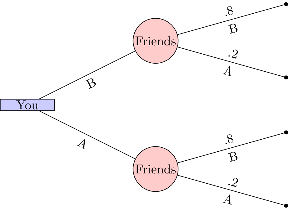
Figure 1:A probabilistic decision tree. A square node is used to indicate a decision and a circlular node is used to indicate a probailistic event.
As illustrated in Figure 1, if you must choose your location without communication, the optimal choice is coffee house B, offering an 80% chance of meeting your friends.
However, in many situations, decisions are not made in isolation. Often, one party moves first, and others respond after observing that choice. If you were able to announce your decision before your friends chose where to go, the interaction would become a sequential decision problem — an instance of a game. Figure 2 shows this game.
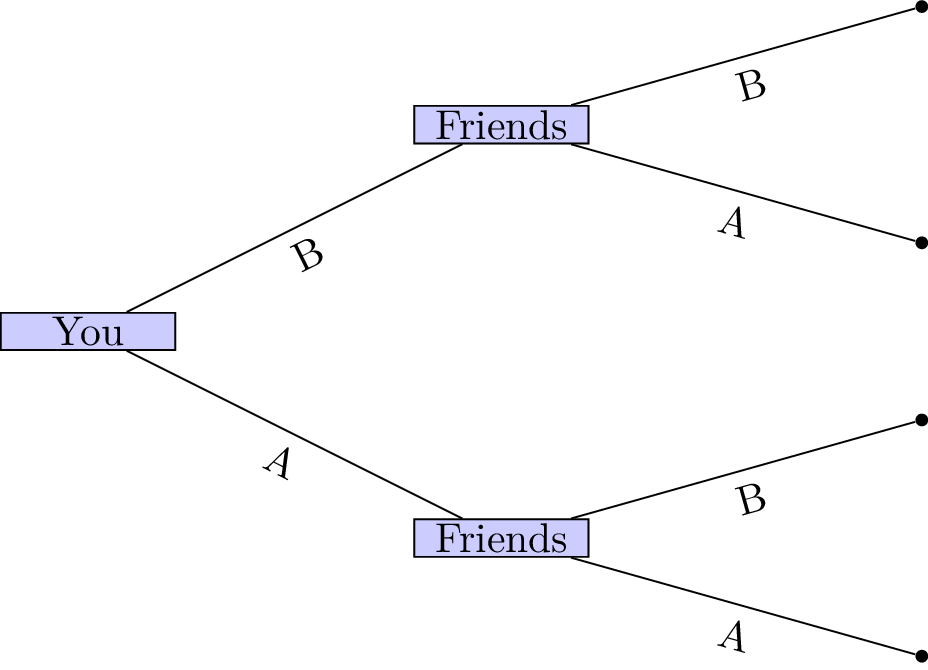
Figure 2:Visual representation of the consecutive decisions.
In such games, outcomes depend not only on chance but critically on the sequence of actions taken by all players.
Theory
We now return to the tree diagrams introduced previously. In game theory, such trees are used to represent a particular type of game known as an extensive form game.
Definition: Extensive Form Game
An -player extensive form game with complete information consists of:
A finite set of players with .
A tree where:
is the set of vertices,
is the set of edges, and
is the root of the tree.
A partition of the non-terminal vertices, assigning each decision node to a player.
A set of possible outcomes.
A function mapping each terminal node (leaf) of to an element of .
Example: Sequential Coordination Game
Consider the following game, often referred to as the Battle of the Sexes.
Two friends must decide which movie to watch at the cinema.
Bob prefers a comedy, while Celine prefers a sports movie.
However, both would rather attend the cinema together than go separately.
The structure of the game and the utilities for Bob and Celine are shown in Figure 3.
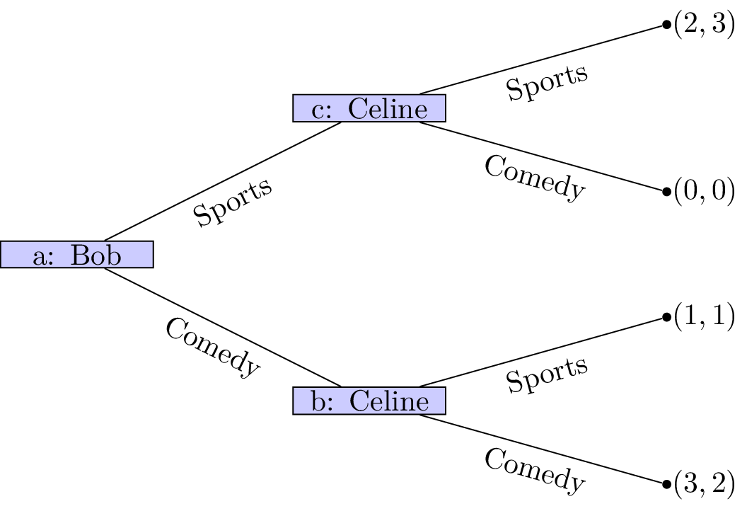
Figure 3:The coordination game with Bob choosing first.
If Bob chooses first, the outcome can be predicted as follows:
Bob observes that whatever choice he makes, Celine will prefer to follow and select the same type of movie.
Bob, anticipating this, chooses a comedy to secure the slightly higher utility he prefers.
(This reasoning uses a method known as backward induction, which we will formalize later.)
Alternatively, we can model the game with Celine moving first, as shown in Figure 4.

Figure 4:The coordination game with Celine choosing first.
In this version:
Celine observes that whatever choice she makes, Bob will prefer to follow and select the same type of movie.
Celine, anticipating this, chooses the sports movie to secure her preferred outcome.
In both representations, we assume that players have complete information about previous actions when making their decisions. Specifically, we assume that the information available at nodes b and c differs: players know precisely where they are in the game. This assumption will later be relaxed when we study games with imperfect information.
Definition: Information Set
Given a game in extensive form
,
the set of information sets for player is a partition
of .
Each element of denotes a set of nodes at which the player cannot distinguish their exact location when choosing an action.
Two nodes of a game tree are said to belong to the same information set if the player making a decision at that point cannot distinguish between them.
This implies that:
Every information set contains vertices for a single player.
All vertices in an information set must have the same number of successors (with the same action labels).
We represent nodes that are part of the same information set diagrammatically by connecting them with a dashed line, as shown in Figure 5.
In our example involving Celine and Bob, if both players must choose a movie without knowing the other’s choice, nodes b and c belong to the same information set.
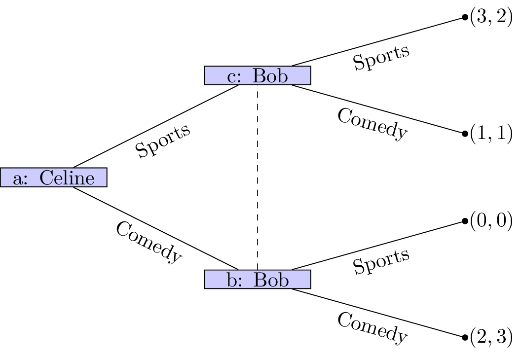
Figure 5:The coordination game with imperfect information.
In this case, it becomes significantly more difficult to predict the outcome of the game.
Another way to represent a game is in normal form.
Definition: Normal Form Game
An -player normal form game consists of:
A finite set of players.
An action set for the players:
.A set of payoff functions for the players:
.
Unless otherwise stated, we assume throughout this text that all players act to maximise their individual payoffs.
Bi-Matrix Representation
One common way to represent a two-player normal form game is using a
bi-matrix. Suppose that and the action sets are:
and
.
A general bi-matrix mapping rows (actions of the first player) and columns (actions of the second player) to pairs of payoff values:
An alternative approach is to use two separate matrices: for the row player and for the column player, defined as follows:
This is the preferred representation used in this text.
Example: Coordination game
The Normal Form Game representation of Figure 5 has the following payoff matrices for the row and column players:
Example: Prisoners’ Dilemma
Two thieves have been caught by the police and separated for questioning.
If both cooperate (remain silent), they each receive a short sentence.
If one defects (betrays the other), they are offered a deal while the other receives a long sentence.
If both defect, they both receive a medium-length sentence.
The normal form of this game is represented by:
Example: Hawk–Dove
Suppose two birds of prey must share a limited resource.
Hawks always fight over the resource — potentially to the death or at great cost — and dominate doves.
Doves, on the other hand, avoid conflict and share the resource if paired with another dove.
This interaction is modelled as:
Example: Pigs
Two pigs — one dominant and one subservient — share a pen containing a lever that dispenses food.
Pressing the lever takes time, giving the other pig an opportunity to eat.
If the dominant pig presses the lever, the subservient pig eats most of the food before being pushed away.
If the subservient pig presses the lever, the dominant pig eats all the food.
If both pigs press the lever, the subservient pig manages to eat a third of the food.
The game is represented by:
Example: Matching Pennies
Two players simultaneously choose to display a coin as either Heads or Tails.
If both players show the same face, player 1 wins.
If the faces differ, player 2 wins.
This zero-sum game is represented as:
We now discuss how players choose their actions in both normal and extensive form games.
Definition: Strategy in Normal Form Games
A strategy for a player with action set is a probability distribution over the elements of .
Typically, a strategy is denoted by , subject to the condition:
Given an action set the set of valid strategies is denoted as so that:
In the Matching Pennies game, a strategy profile such as
and implies that player 1 plays
Heads with probability 0.2, and player 2 plays Heads with probability 0.6.
We can extend the utility function, which maps from action profiles to , using expected utility. For a two-player game, we write:
Here, we treat as a function so that is the probability of choosing action .
Example: Expected Utility in Matching Pennies
Using the Matching Pennies game and the strategy profile
and , the expected utilities are:
Now, suppose player 2 always plays Tails. Then
, and if , we have:
Similarly, if player 1 always plays Tails, and
, the expected utility for player 2 is:
If we simplify and assume player 1 always plays Tails, then and we get:
We can visualise both of these expected utility functions below:
import matplotlib.pyplot as plt
import numpy as np

x = np.linspace(0, 1, 100)

plt.figure()
plt.plot(x, 1 - 2 * x, label="$u_1$ (column plays tails)")
plt.plot(x, 2 * x - 1, label="$u_2$ (row plays tails)")
plt.xlabel("Probability of playing Heads")
plt.ylabel("Expected Utility")
plt.legend()
plt.title("Expected Utility vs Strategy");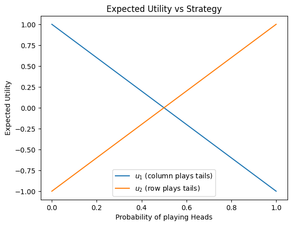
Definition: Strategy in Extensive Form Games
A strategy for a player in an Extensive Form Game is a mapping from each information set to a probability distribution over the available actions at that set.
Example: Strategies in the Sequential Coordination Game
In the Sequential Coordination Game, Bob has a single decision node. His strategy can be represented as:
where is the probability of choosing “sports”.
Celine has two decision nodes, which depend on Bob’s choice. Her strategy is:
Here, is the probability of choosing “sports” if Bob chose sports, and is the probability of choosing sports if Bob chose comedy.
If Celine is unaware of Bob’s decision, as in the
coordination game with imperfect information,
then nodes b and c form a single information set. Her strategy becomes:
This leads us to a fundamental idea: every extensive form game corresponds to a normal form game, where strategies describe complete plans of action across all information sets.
Mapping Extensive Form Games to Normal Form
An extensive form game can be mapped to a normal form game by enumerating all possible strategies that specify a single action at each information set. This collection of strategies defines the action sets in the corresponding normal form game.
These strategies can be thought of as vectors in the Cartesian product of the
action sets available at each information set. For a player
with information sets
, a strategy
prescribes one action at each information set.
For example, specifies the action to take at every vertex contained
within .
Example: Strategy Enumeration in the Sequential Coordination Game
Consider the
Sequential Coordination Game.
We enumerate all strategies for each player by listing single actions
taken at each information set.
For Bob, who has a single information set, the list of all strategies in the extensive form game that prescribe a single action is:
These correspond to always choosing Sports or always choosing Comedy. The action set in the Normal Form Game is:
For Celine, who has two information sets (after Bob’s move), the pure strategies in the extensive form are:
These strategies describe how Celine responds to each of Bob’s possible choices. Thinking of these as vectors in the Cartesian product of available actions at each information set, we can define Celine’s action set in the Normal Form Game as:
Using these enumerated strategies, the payoff matrices for Bob (the row player) and Celine (the column player) are:
Exercises
Programming
Linear Algebraic Form of Expected Utility
The expected utility calculation defined in (10) corresponds to a matrix formulation using linear algebra:
Here, is the payoff matrix for player , and , are row and column player strategies, treated as row vectors.
This linear algebraic form will be important in later chapters, and it also enables efficient numerical computation in programming languages that support vectorized matrix operations.
Using NumPy to Compute Expected Utilities
Python’s numerical library NumPy Harris et al., 2020 provides vectorized operations through
its array class. Below, we define the elements from the
earlier Matching Pennies example:
import numpy as np

M_r = np.array(
    (
        (1, -1),
        (-1, 1),
    )
)
M_c = -M_r

sigma_r = np.array((0.2, 0.8))
sigma_c = np.array((0.6, 0.4))We can now compute the expected utility for the row player using (24):
sigma_r @ M_r @ sigma_cnp.float64(-0.12)The equivalent calculation for the column player is:
sigma_r @ M_c @ sigma_cnp.float64(0.12)Using Nashpy to Create Games and Compute Utilities
The Python library Nashpy Knight & Campbell, 2018 is specifically designed for two-player normal form games. We can use it to create the Matching Pennies game:
import nashpy as nash

matching_pennies = nash.Game(M_r, M_c)
matching_pennies
Zero sum game with payoff matrices:
Row player:
[[ 1 -1]
[-1 1]]
Column player:
[[-1 1]
[ 1 -1]]To compute the expected utilities of both players:
matching_pennies[sigma_r, sigma_c]array([-0.12, 0.12])Creating a 3 player game using Gambit
Here we create a Normal Form game in Gambit Savani & Turocy, 2024 with 3 players:
import pygambit as gbt

g = gbt.Game.new_table([2, 2, 2])
p1, p2, p3 = g.players
Now let us write all the utilities of each outcome:
g[(0, 0, 0)][p1] = 1
g[(0, 0, 0)][p2] = 1
g[(0, 0, 0)][p3] = 1

g[(0, 0, 1)][p1] = 2
g[(0, 0, 1)][p2] = 1
g[(0, 0, 1)][p3] = -1

g[(0, 1, 0)][p1] = 2
g[(0, 1, 0)][p2] = 1
g[(0, 1, 0)][p3] = -1

g[(0, 1, 1)][p1] = 2
g[(0, 1, 1)][p2] = 1
g[(0, 1, 1)][p3] = -1

g[(1, 0, 0)][p1] = 2
g[(1, 0, 0)][p2] = 1
g[(1, 0, 0)][p3] = -1

g[(1, 0, 1)][p1] = 2
g[(1, 0, 1)][p2] = 1
g[(1, 0, 1)][p3] = -1

g[(1, 1, 0)][p1] = 2
g[(1, 1, 0)][p2] = 1
g[(1, 1, 0)][p3] = -1

g[(1, 1, 1)][p1] = 1
g[(1, 1, 1)][p2] = 1
g[(1, 1, 1)][p3] = 1
gNotable Research
This chapter has introduced the mathematical foundations needed to define games and strategic behaviour in interactive decision-making. In later chapters, we will analyse emergent behaviour, a central focus of much contemporary game theory research.
This section presents a brief overview of selected studies that demonstrate how game theory is applied across a range of real-world scenarios. We highlight the types of situations being modelled rather than focusing on technical details.
In Lee & Roberts, 2016, the authors develop a game-theoretic model of rhino horn devaluation—a conservation strategy in which a rhinoceros’s horn is partially removed to reduce its value to poachers. This work, along with follow-up research such as Glynatsi et al., 2018, explores the conditions under which poachers are deterred from targeting these endangered animals.
Game theory has also been applied to healthcare systems. In Knight et al., 2017, hospitals are modelled as agents who may strategically limit bed availability to meet performance targets. A related study, Panayides et al., 2023, examines the interaction between hospitals and ambulance services. Both models use game theory to identify conditions under which rational decision-making may benefit patients overall.
In a different health-related setting, Basanta et al., 2008 presents a game-theoretic model of cancer progression, interpreting the dynamics between different cell types through the lens of evolutionary games.
In Jordan et al., 2009, the authors model play calling in American Football. Their framework incorporates factors such as game stage and risk aversion to identify advantageous strategic decisions in a Normal Form setting.
The study Kwak et al., 2020 constructs a game-theoretic version of the Volunteer’s Dilemma, in which individuals can choose to help or remain bystanders. The authors formalise this as a general -player Normal Form Game and investigate how helping behaviour varies with the cost of intervention.
A related dilemma is explored in Weitz et al., 2016, where the focus shifts from individual help to shared environmental resources. This model examines how agent behaviour affects the environment, which in turn feeds back to influence future strategic choices.
While the above studies are primarily based on Normal Form Games, Boyd et al., 2023 presents a model in Extensive Form. The authors consider a water resource management problem where three firms are located sequentially along a river basin. The model captures the asymmetric benefits faced by upstream versus downstream players. The proposed mechanism—a non-cooperative water-release market—enables upstream agents to release water, creating a more equitable outcome for all parties.
Conclusion
In this chapter, we introduced the formal structure of games, focusing on both normal form and extensive form representations. Table 1 shows a comparison of these two forms. We saw how strategies, utilities, and information sets define the behaviour of rational agents in interactive decision-making scenarios.
Table 1:The main concepts for Normal Form and Extensive Form Games.
| Concept | Normal Form Game | Extensive Form Game |
|---|---|---|
| Representation | Payoff Matrices | Game tree |
| Sequence of Moves | Simultaneous | Sequential (possibly with information sets) |
| Players | ||
| Actions | per player | Specified at each decision node |
| Strategies | Probability distributions over actions | Mappings from information sets to probability distributions over actions |
| Utilities | for action profiles | for each terminal node |
| Information | Perfect (assumes all actions known at once) | Can be perfect or imperfect (via information sets) |
Through motivating examples, formal definitions, and real-world applications, we began to see how even simple games can model complex dynamics. From coordinating with friends to navigating competitive environments, these tools lay the groundwork for deeper analysis in the chapters to come.
Next, we turn to the study of emergent behaviour, where individual strategies interact in surprising ways across repeated play, populations, or networks of agents. Understanding these patterns is essential for analysing systems that evolve over time — and for designing mechanisms that shape them.
- Harris, C. R., Millman, K. J., van der Walt, S. J., Gommers, R., Virtanen, P., Cournapeau, D., Wieser, E., Taylor, J., Berg, S., Smith, N. J., Kern, R., Picus, M., Hoyer, S., van Kerkwijk, M. H., Brett, M., Haldane, A., del Río, J. F., Wiebe, M., Peterson, P., … Oliphant, T. E. (2020). Array programming with NumPy. Nature, 585(7825), 357–362. 10.1038/s41586-020-2649-2
- Knight, V., & Campbell, J. (2018). Nashpy: A Python library for the computation of Nash equilibria. Journal of Open Source Software, 3(30), 904.
- Savani, R., & Turocy, T. L. (2024). Gambit: The package for computation in game theory, Version 16.2. 0.
- Lee, T. E., & Roberts, D. L. (2016). Devaluing rhino horns as a theoretical game. Ecological Modelling, 337, 73–78.
- Glynatsi, N. E., Knight, V., & Lee, T. E. (2018). An evolutionary game theoretic model of rhino horn devaluation. Ecological Modelling, 389, 33–40.
- Knight, V., Komenda, I., & Griffiths, J. (2017). Measuring the price of anarchy in critical care unit interactions. Journal of the Operational Research Society, 68(6), 630–642.
- Panayides, M., Knight, V., & Harper, P. (2023). A game theoretic model of the behavioural gaming that takes place at the EMS-ED interface. European Journal of Operational Research, 305(3), 1236–1258.
- Basanta, D., Hatzikirou, H., & Deutsch, A. (2008). Studying the emergence of invasiveness in tumours using game theory. The European Physical Journal B, 63, 393–397.
- Jordan, J. D., Melouk, S. H., & Perry, M. B. (2009). Optimizing football game play calling. Journal of Quantitative Analysis in Sports, 5(2).
- Kwak, J., Lees, M. H., Cai, W., & Ong, M. E. (2020). Modeling helping behavior in emergency evacuations using volunteer’s dilemma game. Computational Science–ICCS 2020: 20th International Conference, Amsterdam, The Netherlands, June 3–5, 2020, Proceedings, Part I 20, 513–523.
- Weitz, J. S., Eksin, C., Paarporn, K., Brown, S. P., & Ratcliff, W. C. (2016). An oscillating tragedy of the commons in replicator dynamics with game-environment feedback. Proceedings of the National Academy of Sciences, 113(47), E7518–E7525.
- Boyd, N. T., Gabriel, S. A., Rest, G., & Dumm, T. (2023). Generalized Nash equilibrium models for asymmetric, non-cooperative games on line graphs: Application to water resource systems. Computers & Operations Research, 154, 106194.