Motivating Example: Air resistance of a sky diver
An object falling under gravity is often assumed to not be subject air resistance. This give:
This differential equation can be solved to give:
where . This in turn gives the vertical displacement of an object falling as:
which can be solved to give:
where . This is all based on (A1.1) which assumes no air resistance. In fact all objects falling experience a drag coefficient (kg/m). Approximate values of are given in Table A1.1.
Table A1.1:Estimated quadratic drag coefficients for skydiver
| Position | (kg/m) |
|---|---|
| Spread-eagle | 0.42875 |
| Aerodynamic | 0.07718 |
| Parachute | 26.79688 |
To take this coefficient in to account (A1.1) is modified to give:
This equation can in fact not be solved to give a closed form solution. Another approach to be able to compute the trajectory of a skydiver is needed. The approach in question is numerical integration and the specific approach in this appendix is Euler’s method.
Theory
Definition: Euler’s Method
Euler’s Method is a first-order numerical procedure for approximating solutions to initial value problems of the form:
Given a step size , Euler’s Method generates a sequence of approximations by:
starting from the initial condition .
At each step, Euler’s Method uses the slope given by the differential equation at the current point to extrapolate forward by a small time step.
The differential equation defines a slope field in the plane. Euler’s Method approximates the solution curve by connecting short tangent segments. At each step, the next point is found by moving forward along the tangent line to the curve at the current point.
This can be visualized as constructing a polygonal approximation to the true solution curve as shown in Figure A1.1.
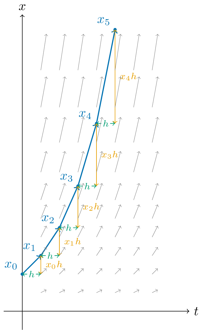
Figure A1.1:A geometric interpretation of numerical integration applied to .
Example: Exponential growth
Consider the differential equation:
The exact solution is .
Applying Euler’s Method with step size gives:
which generates the sequence:
As and with , this approximates .
Exercises
Exercise: Approximating exponential growth
Use Euler’s method to approximate the solution to the differential equation:
with step size up to .
Compute the values of using Euler’s method.
Compare each value to the exact solution at the same time points.
Comment on how the approximation behaves: is it an overestimate or an underestimate? Why?
Exercise: Visualizing Euler’s method
Consider the differential equation:
Use Euler’s method with step size to compute the first 5 steps.
Plot the approximation.
Sketch or describe the qualitative behavior of the true solution.
Exercise: Error and convergence
Let be the true solution to the initial value problem:
Derive the exact solution.
Use Euler’s method with step sizes , 0.25, and 0.125 to compute .
For each step size, compute the absolute error at .
Discuss how the error changes as decreases. What does this suggest about the convergence of Euler’s method?
Programming
Writing an implementation of Euler’s method
The following python function implements Euler’s method:
def get_euler_steps(function, number_of_steps, h, x_0):
    """
    Given a differential equation of the following form:

    dx/dt = function(x)

    This returns `number_of_steps` as given by Euler's algorithm:

    x_{n + 1} = x_n + h function(x_n)

    Parameters
    ----------
    function : A python function -- corresponding to the right hand side of the
               ordinary differential equation
    number_of_steps : int -- The number of iterations of the algorithm
    h : float -- The step size
    x_0 : float -- the initial_value of x

    Returns
    -------
    steps : A python list
    """
    steps = [x_0]
    for _ in range(number_of_steps):
        steps.append(steps[-1] + h * function(steps[-1]))
    return steps
We can use this function to get the steps as required:
def derivative(x):
    return x

number_of_steps = 10
h = 0.1
x_0 = 1
steps = get_euler_steps(
    function=derivative,
    number_of_steps=number_of_steps,
    h=h,
    x_0=x_0,
)
steps
[1,
1.1,
1.2100000000000002,
1.3310000000000002,
1.4641000000000002,
1.61051,
1.7715610000000002,
1.9487171,
2.1435888100000002,
2.357947691,
2.5937424601]Using Scipy’s ordinary differential equation integrator
The Scipy library has an implementation of numerical integration for ordinary differential equations based on an algorithm described in Petzold, 1983. One difference with the previous section is that the function corresponding to the right hand side of the ordinary differential equation must take as an input even if it does not use it and it also takes a sequence of time points instead of a number of steps. Let us start by setting those up:
import scipy.integrate
import numpy as np

def derivative(x, t):
    return x

t = np.linspace(0, 1, 10)
steps = scipy.integrate.odeint(func=derivative, t=t, y0=x_0)
stepsarray([[1. ],
[1.11751906],
[1.24884886],
[1.39561243],
[1.55962349],
[1.742909 ],
[1.94773405],
[2.17663003],
[2.43242551],
[2.7182819 ]])Notable Research
The earliest method of numerical integration, now known as Euler’s method, originates from the foundational work of Leonhard Euler in the 18th century. He implicitly described the approach in Euler, 1768, laying the groundwork for using tangent approximations to solve differential equations numerically.
The natural development from Euler’s idea led to the class of Runge–Kutta methods, which provide higher-order accuracy by sampling the derivative at multiple points. These were introduced independently by Runge Runge, 1895 and Kutta Kutta, 1901, and remain the basis of many modern solvers.
In contemporary settings, attention has turned to the distinction between stiff and non-stiff problems. These require different integration techniques for efficient and stable solutions. Foundational references include Hairer et al., 1993 for non-stiff problems and Hairer & Wanner, 1996 for stiff and differential-algebraic systems.
An important algorithm widely used today is LSODA, described in Petzold, 1983. This method automatically switches between stiff and non-stiff solvers based on the behaviour of the system, and it underpins many solvers, including those in the SciPy library.
Conclusion
Euler’s method offers a simple and intuitive introduction to numerical integration, but it highlights the tradeoff between simplicity, accuracy, and stability. Modern applications often involve stiff systems or demand high accuracy, where more advanced methods are preferable.
[tbl:numerical_methods_summary] summarizes key properties of several commonly used numerical integration methods.
Table A1.2:Summary of numerical methods. Higher-order methods reduce error more quickly with smaller steps. Stiff solvers handle problems where some parts evolve much faster than others.
| Method | Order of Accuracy | Stiff Solver | Notes |
|---|---|---|---|
| Euler | 1 | No | Simple, intuitive |
| RK4 | 4 | No | Widely used, good for smooth ODEs |
| Backward Euler | 1 | Yes | Implicit, stable for stiff systems |
| LSODA | Adaptive | Yes | Switches between stiff/non-stiff |
- Petzold, L. R. (1983). Automatic selection of methods for solving stiff and nonstiff systems of ordinary differential equations. SIAM Journal on Scientific and Statistical Computing, 4(1), 136–148.
- Euler, L. (1768). Institutionum Calculi Integralis. Academiae Imperialis Scientiarum Petropolitanae.
- Runge, C. (1895). Über die numerische Auflösung von Differentialgleichungen. Mathematische Annalen, 46(2), 167–178.
- Kutta, W. (1901). Beiträge zur näherungsweisen Integration totaler Differentialgleichungen. Zeitschrift Für Mathematik Und Physik, 46, 435–453.
- Hairer, E., Nørsett, S. P., & Wanner, G. (1993). Solving Ordinary Differential Equations I: Nonstiff Problems (2nd ed., Vol. 8). Springer.
- Hairer, E., & Wanner, G. (1996). Solving Ordinary Differential Equations II: Stiff and Differential-Algebraic Problems (2nd ed., Vol. 14). Springer.