Motivating Example: Competing Restaurant Locations
Two restaurant chains, FreshBite and UrbanEats, are expanding into a new city. Each must choose one of three neighbourhoods for a flagship store: Downtown, Midtown, or Suburb.
FreshBite (row player) prioritises foot traffic and brand visibility.
UrbanEats (column player) prefers low rental costs and long-term margins.
The projected profits (in £1000s) for each company depend on both their own choice and their competitor’s. Since they are competing in the same market, outcomes reflect strategic interaction.
Table 1 and Table 2 show the expected profits for each company based on their own decision (row) and their competitor’s choice (column).
Table 1:Projected profits for FreshBite (in thousands of pounds)
| Downtown | Midtown | Suburb | |
|---|---|---|---|
| Downtown | 4 | 3 | 2 |
| Midtown | 3 | 2 | 3 |
| Suburb | 2 | 1 | 1 |
Table 2:Projected profits for UrbanEats (in thousands of pounds)
| Downtown | Midtown | Suburb | |
|---|---|---|---|
| Downtown | 1 | 0 | 2 |
| Midtown | 0 | 2 | 6 |
| Suburb | 2 | 4 | 5 |
These tables are assumed to be publicly available from a consultation commissioned by the city council.
The payoff matrices for the equivalent Normal Form Game are:
Let us begin from FreshBite’s perspective: Suburb results in lower profits than Midtown or Downtown, regardless of UrbanEats’ action. A rational FreshBite would therefore never choose Suburb, as illustrated in Figure 1 although it might still choose Midtown or Downtown.
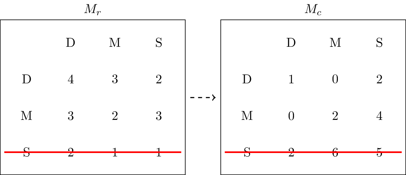
Figure 1:Crossing out Suburb as an action that will never be played by the row player.
With Suburb eliminated for FreshBite, UrbanEats can update their view. Against the remaining options (Downtown and Midtown), UrbanEats consistently receives higher profits by choosing Suburb rather than either alternative. Hence, Downtown and Midtown can be removed from consideration, as shown in Figure 2.
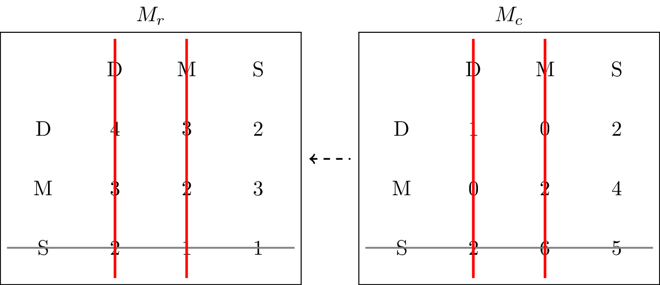
Figure 2:Crossing out Midtown and Downtown as actions that will never be played by the column player.
FreshBite, now comparing Downtown and Midtown against only Suburb from UrbanEats, finds that Midtown yields a better outcome. They therefore eliminate Downtown, leaving Midtown as their only rational option, as shown in Figure 3.
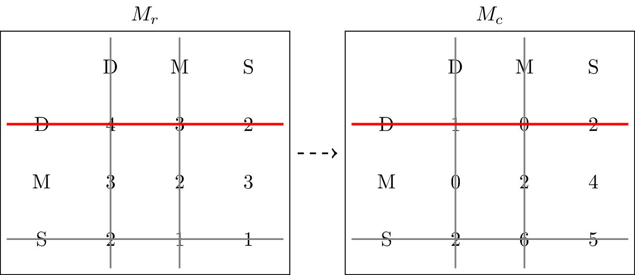
Figure 3:Crossing out Downtown as an action that will never be played by the row player.
The step-by-step logic of iterated elimination of strategies, combined with the assumption of full information and mutual rationality, leads to the predicted outcome:
FreshBite opens in Midtown: with an expected profit of £3,000.
UrbanEats opens in Surbuban: with an expected profit of £4,000
In the next section, we introduce the theory of dominance and best responses. These concepts provide the formal tools for identifying outcomes like this one, and for understanding how strategic agents simplify complex decisions.
Theory
In certain games it is evident that certain strategies should never be used by a rational player. To formalise this we need a couple of definitions.
Definition: Incomplete Strategy Profile
In an -player normal form game, when focusing on player , we denote by an incomplete strategy profile representing the strategies chosen by all players except player .
For example, in a 3-player game where for all , a valid strategy profile might be , indicating that players 1 and 2 choose , and player 3 chooses .
The corresponding incomplete strategy profile for player 2 is: — capturing only the choices of players 1 and 3.
We write to denote the set of all such incomplete strategy profiles from the perspective of player .
This notation allows us to define a key concept in strategic reasoning.
Definition: Strictly Dominated Strategy
In an -player normal form game, an action is said to be strictly dominated if there exists a strategy such that:
That is, no matter what the other players do, player always receives a strictly higher payoff by playing instead of the action .
When modelling rational behaviour, such actions can be systematically excluded from consideration.
Definition: Weakly Dominated Strategy
In an -player normal form game, an action is said to be weakly dominated if there exists a strategy such that:
and
That is, does at least as well as against all possible strategies of the other players, and strictly better against at least one.
As with strictly dominated strategies, we can use weak dominance to guide predictions of rational behaviour by eliminating weakly dominated strategies. Doing so, however, relies on a deeper assumption about what players know about one another.
Common Knowledge of Rationality
So far, we have assumed that players behave rationally. But to justify iterative elimination procedures, we must go further. The key idea is that not only are players rational, but they also know that others are rational—and that this knowledge is shared recursively.
This leads to the concept of Common Knowledge of Rationality (CKR):
Each player is rational.
Each player knows that all other players are rational.
Each player knows that all others know that they are rational.
Each player knows that all others know that they all know that they are rational.
And so on, indefinitely.
This infinite chain of mutual knowledge is what constitutes common knowledge.
By assuming CKR, we justify the use of techniques like the iterated elimination of dominated strategies as a model of rational prediction.
Example: Predicted Behaviour through Iterated Elimination Strategies
Consider the following normal form game, with separate payoff matrices for the row and column players:
We proceed by examining whether any strategies can be removed based on weak dominance.
Step 1: From the column player’s perspective, column is weakly dominated by column . That is, for every row, performs at least as well as , and strictly better for at least one row. We remove from consideration.
Step 2: With removed, the row player now compares and . Row is weakly dominated by , since yields outcomes that are always at least as good and sometimes strictly better. We eliminate .
Step 3: Finally, the column player is left with and . Column is now weakly dominated by , and can be eliminated.
After these steps, we are left with a single strategy profile:
This strategy profile is a predicted outcome based on iterated elimination of weakly dominated strategies, assuming mutual rationality and full knowledge of the payoffs.
Example: eliminating strategies does not suffice
In many cases, we can simplify a game by eliminating dominated strategies. However, not all games can be fully resolved using this approach.
Consider the following game.
Although some weakly dominated strategies may be eliminated here, we still end up with multiple strategy combinations remaining. No single obvious solution emerges from dominance alone. Here is another example:
In this game, no strategy is strictly or weakly dominated for either player. Elimination techniques do not reduce the strategy space, and further analysis is required to predict behaviour.
These examples show that dominance is a helpful tool, but not always sufficient. We need further concepts—such as best responses to analyse such games. Payoff matrices for the row and column players:
Definition: Best Response
In an -player normal form game, a strategy for player is a best response to some incomplete strategy profile if and only if:
That is, gives player the highest possible payoff, given the strategies chosen by the other players.
We can now begin to predict rational behaviour by identifying the best responses to actions of the other players.
Example: Predicted Behaviour through Best Responses in the Action Space
Consider the following game with payoff matrices for the row and column players:
We highlight best responses by underlining the maximum value(s) in each row (for the column player) and in each column (for the row player):
Here, is a pair of best responses:
is a best response to ,
and is a best response to .
This mutual best response suggests a potential stable outcome.
In the next example we will consider finding best responses in the entire strategy space and not just the action space.
Example: Predicted Behaviour through Best Responses in the Strategy Space
We can also identify best responses when players use strategies. Let us begin by examining the Matching Pennies game.
Example: Matching Pennies
Recalling the Payoff matrices for the row and column players:
Assume that player 2 plays a strategy . Then player 1’s expected utilities are:
We will use some code to plot these two payoff values:
import matplotlib.pyplot as plt
import numpy as np

x = np.array((0, 1))

plt.figure()
plt.plot(2 * x - 1, label=r"$u_1(r_1, \sigma_2) = 2x - 1$")
plt.plot(1 -  2 * x, label=r"$ u_1(r_2, \sigma_2) = 1 - 2x $")
plt.title("Utility of the row player's actions as a function of the stratey played by the column player")
plt.xlabel("$x$")
plt.legend();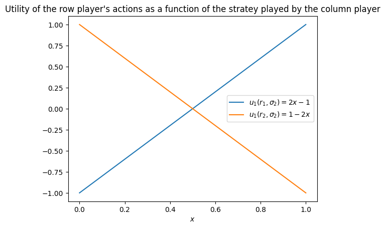
From the graph we observe:
If , then is a best response for player 1.
If , then is a best response for player 1.
If , then player 1 is indifferent between and .
Examples: Coordination Game
Recalling the Payoff matrices for the row and column players:
Assume that player 1 plays a strategy . Then player 2’s expected utilities are:
We will use some code to plot these two payoff values:
import matplotlib.pyplot as plt
import numpy as np

x = np.array((0, 1))

plt.figure()
plt.plot(x + 1, label=r"$u_2(\sigma_1, c_1) = x + 1$")
plt.plot(3 - 3 * x, label=r"$ u_2(\sigma_2, c_2) = 3 - 3 x $")
plt.title("Utility of the column player's actions as a function of the stratey played by the row player")
plt.xlabel("$x$")
plt.legend();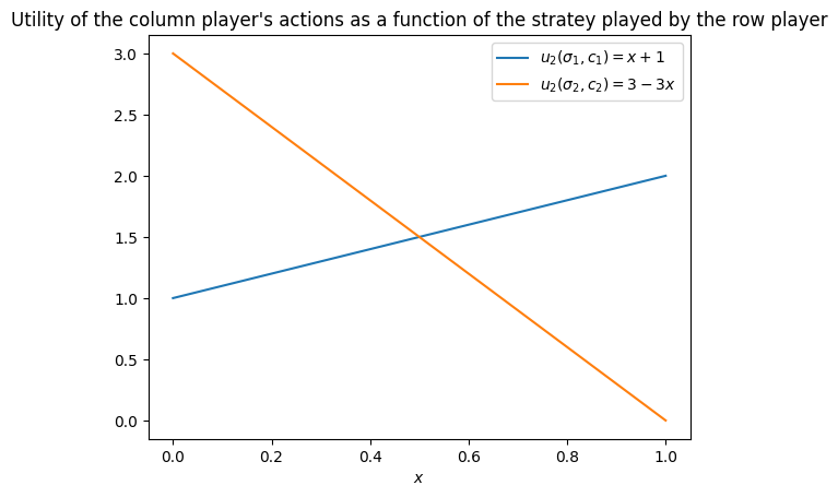
We can now determine the best response for player 1 based on the value of :
If , then is a best response.
If , then is a best response.
If , then player 1 is indifferent between and .
This example shows how best responses depend continuously on the opponent’s strategy, and that indifference can arise at precise thresholds in strategies.
Theorem: Best Response Condition
In a two-player game , a strategy of the row player is a best response to a strategy of the column player if and only if:
Proof
The term represents the utility for the row player when playing their action. Thus:
Let . Then:
Since for all , the maximum expected utility for the row player is , and this occurs if and only if:
as required.
Example: Rock Paper Scissors Lizard Spock
The classic Rock Paper Scissors game can be extended to Rock Paper Scissors Lizard Spock, where:
Scissors cuts Paper
Paper covers Rock
Rock crushes Lizard
Lizard poisons Spock
Spock smashes Scissors
Scissors decapitates Lizard
Lizard eats Paper
Paper disproves Spock
Spock vaporizes Rock
Rock crushes Scissors
This results in the following payoff matrices:
We can now use the Best Response Condition Theorem to check whether the strategy is a best response to .
We begin by computing the expected utilities for each of player 1’s actions:
From this vector, we observe that:
The support of is . Among these, only equals the maximum.
Since and , the condition for a best response is not satisfied.
Therefore, is not a best response to . Indeed, the row player should revise their strategy to place positive weight only on the action that yields the maximum payoff.
Exercises
Programming
Computing utilities of all actions
Theorem: Best Response Condition relies on computing the utilities of all actions when the other player is playing a specific strategy. This corresponds to the matrix multiplication:
Similarly to Linear Algebraic Form of Expected Utility this enables efficient numerical computation in programming languages that support vectorized matrix operations.
Computing utilities of all actions with Numpy
Python’s numerical library NumPy Harris et al., 2020 provides vectorized operations through
its array class. Below, we define the elements from the
earlier Rock Paper Scissors Lizard Spock example:
M_r = np.array(
    (
        (0, -1, 1, 1, -1),
        (1, 0, -1, -1, 1),
        (-1, 1, 0, 1, -1),
        (-1, 1, -1, 0, 1),
        (1, -1, 1, -1, 0),
    )
)

sigma_2 = np.array((1 / 4, 0, 0, 3 / 4, 0))
We can now compute the expected utility for each of the row player’s actions:
M_r @ sigma_2array([ 0.75, -0.5 , 0.5 , -0.25, -0.5 ])Finding non zero entries of an array with Numpy
NumPy gives functionality for finding non zero entries of an array:
sigma_1 = np.array((1 / 3, 0, 1 / 3, 1 / 3, 0))
sigma_1.nonzero()
(array([0, 2, 3]),)Checking the best response condition with Numpy
To check the best response condition with NumPy we can efficiently compare the location of the non zero values of a strategy with the maximum utility of the action set.
(M_r @ sigma_2)[sigma_1.nonzero()] == (M_r @ sigma_2).max()array([ True, False, False])Just as in Example: Rock Paper Scissors Lizard Spock we see that is not a best response as all the non zero values do not give maximum utility. If we modify the row player’s behaviour to only play the first action then we do get a best response:
sigma_1 = np.array((1, 0, 0, 0, 0))
(M_r @ sigma_2)[sigma_1.nonzero()] == (M_r @ sigma_2).max()
array([ True])Checking best response condition with Nashpy
The Python library Nashpy Knight & Campbell, 2018 can be used to directly check the best response condition for two strategies. It checks if either strategy is a best response to each other.
import nashpy as nash

rpsls = nash.Game(M_r, - M_r)
rpsls.is_best_response(sigma_r=sigma_1, sigma_c=sigma_2)
(True, False)This confirms that is a best response to but not vice versa.
Notable Research
In Nash Jr, 1950, John Nash introduced the foundational concept of Nash equilibrium: a strategy profile (i.e., a combination of strategies, one per player) where each strategy is a best response to the others. In such a setting, no player has an incentive to unilaterally deviate from their choice. Nash’s landmark result showed that at least one such equilibrium exists in any finite game — a result that earned him the Nobel Prize in Economics.
More recent research explores how often certain types of equilibria occur. For instance, Wiese & Heinrich, 2022 investigates how frequently best response dynamics (where players iteratively switch to their best response) lead to convergence at a Nash equilibrium. This builds on earlier work such as Dresher, 1970, which studied the likelihood that a game possesses a Nash equilibrium in actions.
Another line of research explores how the structure of a game influences the convergence to equilibrium. For example, in congestion games or routing games, players choose paths through a network, and each player’s cost depends on the congestion caused by others. These games often admit Nash equilibria in actions and allow best response dynamics to converge under mild conditions. This property has led to applications in traffic flow, internet routing, and load balancing. The work of Rosenthal, 1973 formally introduced this class of games and remains a cornerstone of algorithmic game theory.
In an applied context, Knight et al., 2017 models interactions between hospitals under performance-based targets. The authors prove the existence of an equilibrium in actions (as opposed to more general strategies). This finding provides insight into how policy incentives might be structured to align hospital decision-making with public health outcomes.
Conclusion
In this chapter, we introduced fundamental tools for predicting strategic behaviour: dominated strategies, best responses, and the assumption of common knowledge of rationality. These ideas allowed us to identify outcomes that rational players would be unlikely to avoid—such as the elimination of actions that never perform best and the selection of strategies that respond optimally to others.
Using both motivating examples and formal definitions, we saw how iterated elimination and best response analysis can reveal plausible behaviours in one-shot games. We also explored how reasoning about rationality can be extended beyond pure actions to strategies, where probability plays a role in decision-making.
These concepts (summarised in Table 3) lay the foundation for understanding equilibrium—the central concept where players’ strategies mutually reinforce each other. In the next chapter, we formalise this idea, introducing Nash equilibrium and exploring its existence, interpretation, and implications across different types of games.
Table 3:Summary of core concepts introduced in this chapter.
| Concept | Description |
|---|---|
| Dominated Strategy | An action that is always worse than another; never rational to play |
| Iterated Elimination | Sequentially removing dominated strategies to simplify the game |
| Best Response | The strategy that maximises a player’s utility given others’ choices |
| Strategy Profile | A complete specification of strategies for all players |
| Incomplete Strategy Profile | Strategies for all players except one |
| Common Knowledge of Rationality | All players are rational, and know that others are, recursively |
| Best Response Condition | A formal test for optimality in response to a strategy |
- Harris, C. R., Millman, K. J., van der Walt, S. J., Gommers, R., Virtanen, P., Cournapeau, D., Wieser, E., Taylor, J., Berg, S., Smith, N. J., Kern, R., Picus, M., Hoyer, S., van Kerkwijk, M. H., Brett, M., Haldane, A., del Río, J. F., Wiebe, M., Peterson, P., … Oliphant, T. E. (2020). Array programming with NumPy. Nature, 585(7825), 357–362. 10.1038/s41586-020-2649-2
- Knight, V., & Campbell, J. (2018). Nashpy: A Python library for the computation of Nash equilibria. Journal of Open Source Software, 3(30), 904.
- Nash Jr, J. F. (1950). Equilibrium points in n-person games. Proceedings of the National Academy of Sciences, 36(1), 48–49.
- Wiese, S. C., & Heinrich, T. (2022). The frequency of convergent games under best-response dynamics. Dynamic Games and Applications, 1–12.
- Dresher, M. (1970). Probability of a pure equilibrium point in n-person games. Journal of Combinatorial Theory, 8(1), 134–145.
- Rosenthal, R. W. (1973). A class of games possessing pure-strategy Nash equilibria. International Journal of Game Theory, 2(1), 65–67.
- Knight, V., Komenda, I., & Griffiths, J. (2017). Measuring the price of anarchy in critical care unit interactions. Journal of the Operational Research Society, 68(6), 630–642.