Routing Games
Selfish agents choosing routes through a shared network rarely produce the
socially optimal outcome. This chapter studies routing games and the Price of
Anarchy, quantifying how much individual optimisation can degrade collective
performance.
Figure 1: A route only stays quick for as long as few people take it. Once every driver
spots the same shortcut and switches onto it, the shortcut is no quicker than
the road it replaced.
Motivating Example: Competing delivery companies ¶ In a busy city, two rival delivery companies, QuickShip and TurboExpress ,
operate daily distribution routes to deliver packages to the central business
district.
Each company starts from its own warehouse, located in different suburbs on
opposite sides of the city. Every morning, the companies dispatch their fleets
toward the central depot, but must decide how to route their vans:
Each company can take its own dedicated service road to the depot.
Alternatively, both companies can use a shared ring road that offers a
faster connection, but becomes congested as total traffic increases.
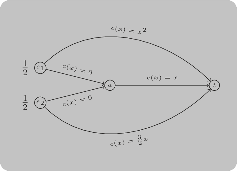
The travel costs for each route depend on the level of congestion:
For QuickShip (source s 1 s_1 s 1
For TurboExpress (source s 2 s_2 s 2
For the shared ring road (available to both companies):
Each source has
a total demand of r = 1 / 2 r = 1 / 2 r = 1/2
This is shown diagrammatically in
Figure 2
Each company decides independently how to distribute its fleet across the
available routes, aiming to minimise its own delivery costs. However, since the
shared road’s cost depends on total usage, each company’s decision affects the
other’s outcome.
This setting creates a routing game , where decentralised decisions lead to
interdependent costs. We will analyse this scenario to explore the concept of
Nash equilibrium in network routing, and investigate how self-interested
routing can result in stable, but potentially inefficient, traffic patterns.
Figure 2: The routes available to QuickShip and TurboExpress.
Theory ¶ Definition: Routing Game ¶ A routing game ( G , r , c ) (G,r,c) ( G , r , c ) G = ( V , E ) G=(V,E) G = ( V , E ) s i s_i s i t i t_i t i r i r_i r i G G G s i s_i s i t i t_i t i e e e G G G c e c_e c e
Example: The Routing Game Representation of the Delivery Companies Game ¶ For the routing game in Figure 2
G = ( V , E ) G=(V, E) G = ( V , E ) V = { s 1 , s 2 , a , t } V=\{s_1, s_2, a, t\} V = { s 1 , s 2 , a , t } E = { ( s 1 , t ) , ( s 1 , a ) , ( s 2 , a ) , ( s 2 , t ) , ( a , t ) } E=\{(s_1, t), (s_1, a), (s_2, a), (s_2, t), (a, t)\} E = {( s 1 , t ) , ( s 1 , a ) , ( s 2 , a ) , ( s 2 , t ) , ( a , t )}
r 1 = r 2 = 1 / 2 r_1=r_2=1/2 r 1 = r 2 = 1/2
c s 1 , t ( x ) = x 2 , c s 2 , t ( x ) = 3 x / 2 , c a , t ( x ) = x , c s 1 , a ( x ) = c s 2 , a = 0 c_{s_1, t}(x)=x^2, c_{s_2, t}(x)=3x/2, c_{a, t}(x)=x, c_{s_1, a}(x)=c_{s_2, a}=0 c s 1 , t ( x ) = x 2 , c s 2 , t ( x ) = 3 x /2 , c a , t ( x ) = x , c s 1 , a ( x ) = c s 2 , a = 0
Definition: Set of Paths ¶ For any given ( G , r , c ) (G,r,c) ( G , r , c ) P i \mathcal{P}_i P i i i i
Definition: Feasible Flow ¶ On a routing game we define a flow f f f f f f P \mathcal{P} P f f f feasible if:
∑ P ∈ P i f P = r i \sum_{P\in\mathcal{P}_i}f_P=r_i P ∈ P i ∑ f P = r i Example: Feasible Flows for the Delivery Companies Game ¶ For the routing game in Figure 2
P 1 = { ( s 1 , a , t ) , ( s 1 , t ) } \mathcal{P}_1=\{(s_1,a,t),(s_1,t)\} P 1 = {( s 1 , a , t ) , ( s 1 , t )} and
P 2 = { ( s 2 , a , t ) , ( s 2 , t ) } \mathcal{P}_2=\{(s_2,a,t),(s_2,t)\} P 2 = {( s 2 , a , t ) , ( s 2 , t )} The set of all possible paths is denoted by P = ∪ i P i \mathcal{P}=\cup_{i}\mathcal{P}_i P = ∪ i P i
Definition: Cost function ¶ For any routing game ( G , r , c ) (G,r,c) ( G , r , c ) cost function C ( f ) C(f) C ( f )
C ( f ) = ∑ P ∈ P c P ( f P ) f P C(f)=\sum_{P\in\mathcal{P}}c_P(f_P)f_P C ( f ) = P ∈ P ∑ c P ( f P ) f P Where c P c_P c P P P P c P ( x ) = ∑ e ∈ P c e ( x ) c_P(x)=\sum_{e\in P}c_e(x) c P ( x ) = ∑ e ∈ P c e ( x ) f f f
f e = ∑ P ∈ P if e ∈ P f P f_e=\sum_{P\in\mathcal{P}\text{ if }e\in P}f_P f e = P ∈ P if e ∈ P ∑ f P So we can re-write the cost function as:
C ( f ) = ∑ e ∈ E c e ( f e ) f e C(f)=\sum_{e\in E}c_e(f_e)f_e C ( f ) = e ∈ E ∑ c e ( f e ) f e Example: Cost function for the Delivery Companies Game ¶ For the routing game in Figure 2
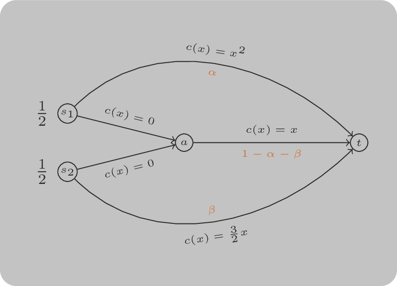
Let f = ( α , 1 / 2 − α , 1 / 2 − β , β ) f=(\alpha,1/2-\alpha,1/2-\beta,\beta) f = ( α , 1/2 − α , 1/2 − β , β ) Figure 3
Figure 3: The vector f f f
The cost of f ( α , 1 / 2 − α , 1 / 2 − β , β ) f(\alpha,1/2-\alpha,1/2-\beta,\beta) f ( α , 1/2 − α , 1/2 − β , β )
C ( f ) = α 2 × α + 3 / 2 β × β + ( 1 − α − β ) × ( 1 − α − β ) = α 3 + 3 / 2 β 2 + α 2 + 2 α β + β 2 − 2 α − 2 β + 1 \begin{align*}
C(f)&=\alpha^2\times\alpha+3/2\beta\times\beta+(1-\alpha-\beta)\times(1-\alpha-\beta)\\
&=\alpha^3+3/2\beta^2+\alpha^2 + 2\alpha\beta + \beta^2 - 2\alpha - 2\beta + 1
\end{align*} C ( f ) = α 2 × α + 3/2 β × β + ( 1 − α − β ) × ( 1 − α − β ) = α 3 + 3/2 β 2 + α 2 + 2 α β + β 2 − 2 α − 2 β + 1 Definition: Optimal Flow ¶ For a routing game ( G , r , c ) (G,r,c) ( G , r , c ) f ∗ f^* f ∗
Minimise ∑ e ∈ E c e ( f e ) f e \sum_{e\in E}c_e(f_e)f_e ∑ e ∈ E c e ( f e ) f e
Subject to:
∑ P ∈ P i f P = r i for all i f e = ∑ P ∈ P if e ∈ P f P for all e ∈ E f P ≥ 0 \begin{align*}
\sum_{P\in\mathcal{P}_i}f_P&=r_i&&\text{for all }i\\
f_e&=\sum_{P\in\mathcal{P}\text{ if }e\in P}f_P&&\text{ for all }e\in E\\
f_P&\geq 0
\end{align*} P ∈ P i ∑ f P f e f P = r i = P ∈ P if e ∈ P ∑ f P ≥ 0 for all i for all e ∈ E Example: Optimal Flow for the Delivery Companies Games ¶ In Figure 3
Minimise C ( α , β ) = α 3 + 3 / 2 β 2 + α 2 + 2 α β + β 2 − 2 α − 2 β + 1 C(\alpha,\beta)=\alpha^3+3/2\beta^2+\alpha^2 + 2\alpha\beta + \beta^2 - 2\alpha - 2\beta + 1 C ( α , β ) = α 3 + 3/2 β 2 + α 2 + 2 α β + β 2 − 2 α − 2 β + 1
Subject to:
0 ≤ α α ≤ 1 / 2 0 ≤ β β ≤ 1 / 2 \begin{align*}
0&\leq\alpha\\
\alpha&\leq 1/2\\
0&\leq\beta\\
\beta&\leq1/2
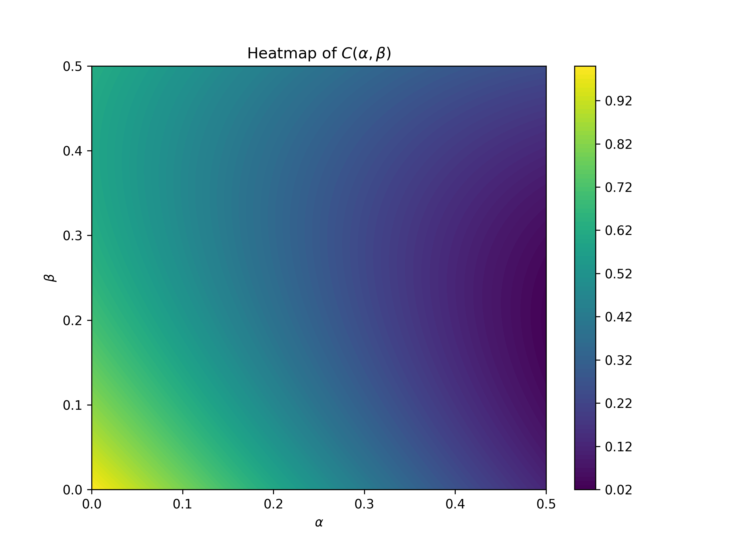
\end{align*} 0 α 0 β ≤ α ≤ 1/2 ≤ β ≤ 1/2 A plot of C ( α , β ) C(\alpha,\beta) C ( α , β ) Figure 4
Figure 4: The plot of ( α , β ) (\alpha, \beta) ( α , β )
The minimal point looks to be near the right boundary of the square, although it
is unclear if it is on the boundary or not. It is in fact not on the
boundary
taking this fact as an assumption, identity the optimal flow using the
Karush-Kuhn-Tucker conditions .
Let us first define the Lagrangian:
L ( α , β , λ ) = C ( α , β ) − λ 1 α − λ 2 ( α − 1 / 2 ) − λ 3 β − λ 4 β \mathcal{L}(\alpha,\beta,\lambda)=C(\alpha,\beta)-\lambda_1\alpha-\lambda_2(\alpha-1/2)-\lambda_3\beta-\lambda_4\beta L ( α , β , λ ) = C ( α , β ) − λ 1 α − λ 2 ( α − 1/2 ) − λ 3 β − λ 4 β If f ∗ f^* f ∗ λ i = 0 \lambda_i=0 λ i = 0 i i i g i ( f ∗ ) = 0 g_i(f^*)=0 g i ( f ∗ ) = 0
Thus:
L ( α , β , λ ) = C ( α , β ) \mathcal{L}(\alpha,\beta,\lambda)=C(\alpha,\beta) L ( α , β , λ ) = C ( α , β ) We note that the feasiblity constraints all hold for f ∗ f^* f ∗
∂ L ∂ α = ∂ C ∂ α = 3 α 2 − 2 ( 1 − α − β ) = 0 \frac{\partial \mathcal{L}}{\partial \alpha}=\frac{\partial C}{\partial \alpha}=3\alpha^2-2(1-\alpha-\beta)=0 ∂ α ∂ L = ∂ α ∂ C = 3 α 2 − 2 ( 1 − α − β ) = 0 and
∂ L ∂ α = ∂ C ∂ β = 3 β − 2 ( 1 − α − β ) = 0 \frac{\partial \mathcal{L}}{\partial \alpha}=\frac{\partial C}{\partial \beta}=3\beta-2(1-\alpha-\beta)=0 ∂ α ∂ L = ∂ β ∂ C = 3 β − 2 ( 1 − α − β ) = 0 which gives:
β = 2 ( 1 − α ) 5 \beta=\frac{2(1-\alpha)}{5} β = 5 2 ( 1 − α ) Substituting this in to the first equation gives:
3 α 2 − 6 / 5 ( 1 − α ) = 0 3\alpha^2-6/5(1-\alpha)=0 3 α 2 − 6/5 ( 1 − α ) = 0 which has solutions:
{ − 1 5 − 11 5 , 11 5 − 1 5 } \left\{- \frac{1}{5} - \frac{\sqrt{11}}{5}, \; \frac{\sqrt{11}}{5} - \frac{1}{5}\right\} { − 5 1 − 5 11 , 5 11 − 5 1 } Only one of those is positive satisfying the constraints, substituting it in to
(14)
β = 12 25 − 2 11 25 \beta=\frac{12}{25} - \frac{2 \sqrt{11}}{25} β = 25 12 − 25 2 11 thus the optimal flow is:
f ∗ = ( 11 5 − 1 5 , 12 25 − 2 11 25 ) f^* = \left(\frac{\sqrt{11}}{5} - \frac{1}{5}, \; \frac{12}{25} - \frac{2 \sqrt{11}}{25}\right) f ∗ = ( 5 11 − 5 1 , 25 12 − 25 2 11 ) If we take a closer look at f ∗ f^* f ∗ ( s 1 , t ) (s_1, t) ( s 1 , t ) ( s 1 , a , t ) (s_1, a, t) ( s 1 , a , t )
C s 1 , t ( f ∗ ) = 12 25 − 2 11 25 ≈ 0.2146 C_{s_1, t}(f^*)=\frac{12}{25} - \frac{2 \sqrt{11}}{25}\approx 0.2146 C s 1 , t ( f ∗ ) = 25 12 − 25 2 11 ≈ 0.2146 The cost along the second path is given by:
C s 1 , a , t ( f ∗ ) = 18 25 − 3 11 25 ≈ 0.3220 C_{s_1, a, t}(f^*)=\frac{18}{25} - \frac{3 \sqrt{11}}{25}\approx 0.3220 C s 1 , a , t ( f ∗ ) = 25 18 − 25 3 11 ≈ 0.3220 Thus traffic going along the second path is experiencing a higher cost. In
practice, they would deviate some of their traffic from the second path to the
first.
This leads to the definition of a Nash flow.
Definition: Nash Flow ¶ For a routing game ( G , r , c ) (G,r,c) ( G , r , c ) f ~ \tilde f f ~ Nash flow
if and only if for every commodity i i i P 1 , P 2 ∈ P _ i P_1,P_2\in\mathcal{P}\_i P 1 , P 2 ∈ P _ i f _ P 1 > 0 f\_{P_1}>0 f _ P 1 > 0
c P 1 ( f ) ≤ c P 2 ( f ) c_{P_1}(f)\leq c_{P_2}(f) c P 1 ( f ) ≤ c P 2 ( f ) A Nash flow ensures that all used paths have minimal costs.
Example: Nash Flow for Delivery companies game ¶ For Figure 3
α 2 = 1 − α − β 3 β 2 = 1 − α − β \begin{aligned}
\alpha^2&=1-\alpha-\beta\\
\frac{3\beta}{2}&=1-\alpha-\beta
\end{aligned} α 2 2 3 β = 1 − α − β = 1 − α − β Solving this gives: β = 2 5 ( 1 − α ) \beta=\frac{2}{5}(1-\alpha) β = 5 2 ( 1 − α ) ⇒ \Rightarrow ⇒ x 2 + 3 5 x − 3 5 x^{2} + \frac{3}{5} x - \frac{3}{5} x 2 + 5 3 x − 5 3
{ − 3 10 − 69 10 , − 3 10 + 69 10 } \left\{- \frac{3}{10} - \frac{\sqrt{69}}{10}, - \frac{3}{10} + \frac{\sqrt{69}}{10}\right\} { − 10 3 − 10 69 , − 10 3 + 10 69 } Neither of these two values are within our region thus there is no Nash flow
where all paths are used.
Let us assume that α = 1 / 2 \alpha=1/2 α = 1/2 P s 1 , a , t P_{s_1, a, t} P s 1 , a , t
3 2 β = 1 2 − β ⇒ β = 1 5 \frac{3}{2}\beta=\frac{1}{2}-\beta\Rightarrow\beta=\frac{1}{5} 2 3 β = 2 1 − β ⇒ β = 5 1 Thus we have f ~ = ( 1 / 2 , 1 / 5 ) \tilde f=(1/2,1/5) f ~ = ( 1/2 , 1/5 ) C ( f ~ ) = 11 / 40 C(\tilde f)=11/40 C ( f ~ ) = 11/40
What if we had assumed that β = 1 / 2 \beta=1/2 β = 1/2
This would have given α 2 = 1 / 2 − α \alpha^2=1/2-\alpha α 2 = 1/2 − α
{ − 1 2 + 3 2 , − 3 2 − 1 2 } \left\{- \frac{1}{2} + \frac{\sqrt{3}}{2}, - \frac{\sqrt{3}}{2} - \frac{1}{2}\right\} { − 2 1 + 2 3 , − 2 3 − 2 1 } Taking the first value for α \alpha α P s 2 , a , t P_{s_2, a, t} P s 2 , a , t P s 2 , t P_{s_2, t} P s 2 , t f ~ = ( 1 / 2 , 1 / 5 ) \tilde f=(1/2,1/5) f ~ = ( 1/2 , 1/5 )
Definition: Potential Function ¶ Given a routing game ( G , r , c ) (G,r,c) ( G , r , c ) potential function of a flow as:
Φ ( f ) = ∑ e ∈ E ∫ 0 f e c e ( x ) d x \Phi(f)=\sum_{e\in E}\int_0^{f_e}c_e(x)dx Φ ( f ) = e ∈ E ∑ ∫ 0 f e c e ( x ) d x Example: Potential Function for the delivery company game ¶ The potential function for Figure 3
Φ ( ( α , β ) ) = ∫ 0 α x 2 d x + ∫ 0 1 − α − β x d x + ∫ 0 β 3 / 2 x d x = α 3 3 + 3 β 2 4 + ( 1 − α − β ) 2 2 \begin{align*}
\Phi((\alpha,\beta))&=\int_0^{\alpha}x^2dx + \int_0^{1-\alpha - \beta}xdx + \int_0^{\beta}3/2xdx\\
&=\frac{\alpha^3}{3}+\frac{3\beta^2}{4}+\frac{(1-\alpha-\beta)^2}{2}
\end{align*} Φ (( α , β )) = ∫ 0 α x 2 d x + ∫ 0 1 − α − β x d x + ∫ 0 β 3/2 x d x = 3 α 3 + 4 3 β 2 + 2 ( 1 − α − β ) 2 Theorem: Nash Flow minimises the potential function ¶ A feasible flow f ~ \tilde f f ~ ( G , r , c ) (G,r,c) ( G , r , c ) Φ ( f ) \Phi(f) Φ ( f )
We state this result without proof. It follows from the first-order (KKT)
optimality conditions for minimising the potential Φ \Phi Φ KKT conditions are the tool used to check
particular flows in the exercises below.
Definition: Marginal Cost ¶ If c c c marginal cost function c ∗ c^* c ∗
c ∗ = d d x ( x c ( x ) ) c^* = \frac{d}{dx}\left(x c(x)\right) c ∗ = d x d ( x c ( x ) ) Example: The marginal costs for the delivery company game ¶ The marginal costs for Figure 3
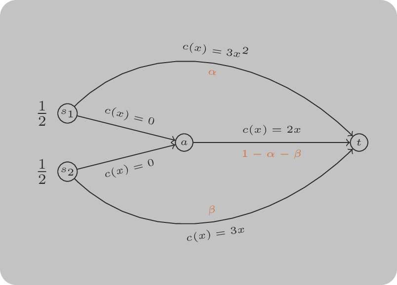
c s 1 , t ∗ ( x ) = 3 x 2 , c s 2 , t ( x ) = 3 x , c a , t ( x ) = 2 x , c s 1 , a ( x ) = c s 2 , a = 0 c^*_{s_1, t}(x)=3x^2, c_{s_2, t}(x)=3x, c_{a, t}(x)=2x, c_{s_1, a}(x)=c_{s_2, a}=0 c s 1 , t ∗ ( x ) = 3 x 2 , c s 2 , t ( x ) = 3 x , c a , t ( x ) = 2 x , c s 1 , a ( x ) = c s 2 , a = 0
The corresponding routing game ( G , r , c ∗ ) (G, r, c^*) ( G , r , c ∗ ) Figure 5
Figure 5: The routes available to QuickShip and TurboExpress with marginal costs instead
of costs.
Theorem: Optimal Flow is a Nash Flow for Marginal Costs ¶ A feasible flow f ∗ f^* f ∗ ( G , r , c ) (G,r,c) ( G , r , c ) f ∗ f^* f ∗ ( G , r , c ∗ ) (G,r,c^*) ( G , r , c ∗ )
We state this result without proof. It follows on comparing the optimality
conditions for the two problems: the optimal flow minimises the total cost
C ( f ) = ∑ e f e c e ( f e ) C(f) = \sum_e f_e c_e(f_e) C ( f ) = ∑ e f e c e ( f e ) c e ∗ = d d x ( x c e ( x ) ) c^*_e = \tfrac{d}{dx}(x c_e(x)) c e ∗ = d x d ( x c e ( x )) c ∗ c^* c ∗
Exercises ¶ Programming ¶ Scipy has functionality for optimising function within certain boundaries,
thanks to Theorem: Nash Flow minimises the potential function
In Appendix: Karush-Kuhn-Tucker Conditions is an example showing how to use Scipy to optimise a
function. Here is another one:
import numpy as np
import scipy.optimize

def objective(f):
    alpha, beta = f
    return alpha ** 3 / 3 + 3 * beta ** 2 / 4 + (1 - alpha - beta) ** 2 / 2

def g_1(f):
    return f[0]

def g_2(f):
    return f[1]

def g_3(f):
    return 1 / 2 - f[0]

def g_4(f):
    return 1 / 2 - f[1]

constraints = [
    {'type': 'ineq', 'fun': g_1},
    {'type': 'ineq', 'fun': g_2},
    {'type': 'ineq', 'fun': g_3},
    {'type': 'ineq', 'fun': g_4},
]

res = scipy.optimize.minimize(objective, [0, 0], constraints=constraints)
print(res)
message: Optimization terminated successfully
success: True
status: 0
fun: 0.11666666666666675
x: [ 5.000e-01 2.000e-01]
nit: 4
jac: [-5.000e-02 -9.313e-10]
nfev: 12
njev: 4
multipliers: [ 0.000e+00 0.000e+00 5.000e-02 0.000e+00]
Notable Research ¶ The original paper introducing the notion of Nash flows is
Wardrop, 1952 Braess’s Paradox Braess, 1968 Steinberg & Zangwill, 1983 Youn et al. , 2008
The inefficiencies that arise in congestion networks due to self-interested
behaviour have led to the concept of the Price of Anarchy , defined as
C ( f ~ ) / C ( f ∗ ) C(\tilde f)/C(f^*) C ( f ~ ) / C ( f ∗ ) Roughgarden & Tardos, 2002 Knight & Harper, 2013
Conclusion ¶ Table 1
Table 1: Summary of routing games
Concept Definition Feasible Flow Any flow satisfying demand and non-negativity constraints Optimal Flow (f ∗ f^* f ∗ Flow minimizing the total system cost $C(f)$ Nash Flow (f ~ \tilde f f ~ Flow where no player can reduce their cost by unilaterally switching routes Potential Function Φ ( f ) = ∑ e ∈ E ∫ 0 f e c e ( x ) d x \Phi(f)=\sum_{e\in E}\int_0^{f_e} c_e(x) dx Φ ( f ) = ∑ e ∈ E ∫ 0 f e c e ( x ) d x Marginal Cost c ∗ ( x ) = d d x ( x c ( x ) ) c^*(x) = \frac{d}{dx}(x c(x)) c ∗ ( x ) = d x d ( x c ( x ))
Solutions ¶ Network without the super road
The network in Figure 6 s s s t t t a a a b b b r = 1 r=1 r = 1
c s , a ( x ) = x , c a , t ( x ) = 1 , c s , b ( x ) = 1 , c b , t ( x ) = x c_{s,a}(x)=x,\quad c_{a,t}(x)=1,\quad c_{s,b}(x)=1,\quad c_{b,t}(x)=x c s , a ( x ) = x , c a , t ( x ) = 1 , c s , b ( x ) = 1 , c b , t ( x ) = x Let α \alpha α P 1 = ( s , a , t ) P_1=(s,a,t) P 1 = ( s , a , t ) 1 − α 1-\alpha 1 − α P 2 = ( s , b , t ) P_2=(s,b,t) P 2 = ( s , b , t ) 0 ≤ α ≤ 1 0\leq\alpha\leq 1 0 ≤ α ≤ 1
Optimal flow (without super road)
The cost function is:
C ( α ) = c s , a ( α ) ⋅ α + c a , t ( α ) ⋅ α + c s , b ( 1 − α ) ⋅ ( 1 − α ) + c b , t ( 1 − α ) ⋅ ( 1 − α ) C(\alpha)=c_{s,a}(\alpha)\cdot\alpha + c_{a,t}(\alpha)\cdot\alpha + c_{s,b}(1-\alpha)\cdot(1-\alpha) + c_{b,t}(1-\alpha)\cdot(1-\alpha) C ( α ) = c s , a ( α ) ⋅ α + c a , t ( α ) ⋅ α + c s , b ( 1 − α ) ⋅ ( 1 − α ) + c b , t ( 1 − α ) ⋅ ( 1 − α ) C ( α ) = α 2 + α + ( 1 − α ) + ( 1 − α ) 2 = α 2 + ( 1 − α ) 2 + 1 C(\alpha)=\alpha^2+\alpha+(1-\alpha)+(1-\alpha)^2=\alpha^2+(1-\alpha)^2+1 C ( α ) = α 2 + α + ( 1 − α ) + ( 1 − α ) 2 = α 2 + ( 1 − α ) 2 + 1 To minimise, take the derivative and set it to zero:
d C d α = 2 α − 2 ( 1 − α ) = 4 α − 2 = 0 ⟹ α ∗ = 1 2 \frac{dC}{d\alpha}=2\alpha-2(1-\alpha)=4\alpha-2=0\implies\alpha^*=\frac{1}{2} d α d C = 2 α − 2 ( 1 − α ) = 4 α − 2 = 0 ⟹ α ∗ = 2 1 The optimal flow is f ∗ = α ∗ = 1 / 2 f^*=\alpha^*=1/2 f ∗ = α ∗ = 1/2
C ( f ∗ ) = 1 4 + 1 4 + 1 = 3 2 C(f^*)=\frac{1}{4}+\frac{1}{4}+1=\frac{3}{2} C ( f ∗ ) = 4 1 + 4 1 + 1 = 2 3 Nash flow (without super road)
A Nash flow requires the cost along every used path to be equal. The cost along each path at flow ( α , 1 − α ) (\alpha, 1-\alpha) ( α , 1 − α )
c P 1 ( α ) = α + 1 , c P 2 ( 1 − α ) = 1 + ( 1 − α ) = 2 − α c_{P_1}(\alpha)=\alpha+1,\qquad c_{P_2}(1-\alpha)=1+(1-\alpha)=2-\alpha c P 1 ( α ) = α + 1 , c P 2 ( 1 − α ) = 1 + ( 1 − α ) = 2 − α Setting c P 1 = c P 2 c_{P_1}=c_{P_2} c P 1 = c P 2
α + 1 = 2 − α ⟹ α ~ = 1 2 \alpha+1=2-\alpha\implies \tilde\alpha=\frac{1}{2} α + 1 = 2 − α ⟹ α ~ = 2 1 So the Nash flow is f ~ = 1 / 2 \tilde f = 1/2 f ~ = 1/2 f ~ = f ∗ \tilde f = f^* f ~ = f ∗
C ( f ~ ) = 3 2 C(\tilde f)=\frac{3}{2} C ( f ~ ) = 2 3 In this case the Nash flow coincides with the optimal flow, so the Price of Anarchy is 1.
import numpy as np
import scipy.optimize

def cost_without_super_road(f):
    alpha = f[0]
    return alpha ** 2 + (1 - alpha) ** 2 + 1

def potential_without_super_road(f):
    alpha = f[0]
    # Phi = int_0^alpha x dx + int_0^alpha 1 dx + int_0^(1-alpha) 1 dx + int_0^(1-alpha) x dx
    return alpha ** 2 / 2 + alpha + (1 - alpha) + (1 - alpha) ** 2 / 2

constraints = [
    {'type': 'ineq', 'fun': lambda f: f[0]},
    {'type': 'ineq', 'fun': lambda f: 1 - f[0]},
]

res_opt = scipy.optimize.minimize(cost_without_super_road, [0.5], constraints=constraints)
res_nash = scipy.optimize.minimize(potential_without_super_road, [0.5], constraints=constraints)

print(f"Optimal flow alpha = {res_opt.x[0]:.4f}, cost = {res_opt.fun:.4f}")
print(f"Nash flow alpha = {res_nash.x[0]:.4f}, cost = {cost_without_super_road(res_nash.x):.4f}")
Optimal flow alpha = 0.5000, cost = 1.5000
Nash flow alpha = 0.5000, cost = 1.5000
Network with the super road (Braess’s Paradox)
The network in Figure 7 a → b a\to b a → b c a , b ( x ) = 0 c_{a,b}(x)=0 c a , b ( x ) = 0 α \alpha α a a a s s s β \beta β a → b a\to b a → b
P 1 = ( s , a , t ) P_1=(s,a,t) P 1 = ( s , a , t ) α − β \alpha-\beta α − β
P 2 = ( s , b , t ) P_2=(s,b,t) P 2 = ( s , b , t ) 1 − α + β 1-\alpha+\beta 1 − α + β
P 3 = ( s , a , b , t ) P_3=(s,a,b,t) P 3 = ( s , a , b , t ) β \beta β
with constraints 0 ≤ β ≤ α 0\leq\beta\leq\alpha 0 ≤ β ≤ α 0 ≤ α ≤ 1 0\leq\alpha\leq 1 0 ≤ α ≤ 1 0 ≤ 1 − α + β ≤ 1 0\leq 1-\alpha+\beta\leq 1 0 ≤ 1 − α + β ≤ 1
The edge flows are: f s , a = α f_{s,a}=\alpha f s , a = α f a , t = α − β f_{a,t}=\alpha-\beta f a , t = α − β f s , b = 1 − α f_{s,b}=1-\alpha f s , b = 1 − α f b , t = 1 − α + β f_{b,t}=1-\alpha+\beta f b , t = 1 − α + β f a , b = β f_{a,b}=\beta f a , b = β
The cost function is:
C ( α , β ) = c s , a ( α ) ⋅ α + c a , t ( α − β ) ⋅ ( α − β ) + c s , b ( 1 − α ) ⋅ ( 1 − α ) + c b , t ( 1 − α + β ) ⋅ ( 1 − α + β ) + c a , b ( β ) ⋅ β = α 2 + ( α − β ) + 1 ⋅ ( 1 − α ) + ( 1 − α + β ) 2 + 0 \begin{align*}
C(\alpha,\beta)&=c_{s,a}(\alpha)\cdot\alpha + c_{a,t}(\alpha-\beta)\cdot(\alpha-\beta)\\
&\quad+c_{s,b}(1-\alpha)\cdot(1-\alpha)+c_{b,t}(1-\alpha+\beta)\cdot(1-\alpha+\beta)\\
&\quad+c_{a,b}(\beta)\cdot\beta\\
&=\alpha^2+(\alpha-\beta)+1\cdot(1-\alpha)+(1-\alpha+\beta)^2+0
\end{align*} C ( α , β ) = c s , a ( α ) ⋅ α + c a , t ( α − β ) ⋅ ( α − β ) + c s , b ( 1 − α ) ⋅ ( 1 − α ) + c b , t ( 1 − α + β ) ⋅ ( 1 − α + β ) + c a , b ( β ) ⋅ β = α 2 + ( α − β ) + 1 ⋅ ( 1 − α ) + ( 1 − α + β ) 2 + 0 Optimal flow (with super road)
The potential function is:
Φ ( α , β ) = α 2 2 + ( α − β ) + ( α − β ) 2 2 ⋅ 0 + ( 1 − α ) + ( 1 − α + β ) 2 2 + 0 \Phi(\alpha,\beta)=\frac{\alpha^2}{2}+(\alpha-\beta)+\frac{(\alpha-\beta)^2}{2}\cdot 0+(1-\alpha)+\frac{(1-\alpha+\beta)^2}{2}+0 Φ ( α , β ) = 2 α 2 + ( α − β ) + 2 ( α − β ) 2 ⋅ 0 + ( 1 − α ) + 2 ( 1 − α + β ) 2 + 0 More carefully, since c s , a ( x ) = x c_{s,a}(x)=x c s , a ( x ) = x c a , t ( x ) = 1 c_{a,t}(x)=1 c a , t ( x ) = 1 c s , b ( x ) = 1 c_{s,b}(x)=1 c s , b ( x ) = 1 c b , t ( x ) = x c_{b,t}(x)=x c b , t ( x ) = x c a , b ( x ) = 0 c_{a,b}(x)=0 c a , b ( x ) = 0
Φ ( α , β ) = α 2 2 + ( α − β ) ⋅ 1 + ( 1 − α ) ⋅ 1 + ( 1 − α + β ) 2 2 \Phi(\alpha,\beta)=\frac{\alpha^2}{2}+({\alpha-\beta})\cdot 1 + (1-\alpha)\cdot 1+\frac{(1-\alpha+\beta)^2}{2} Φ ( α , β ) = 2 α 2 + ( α − β ) ⋅ 1 + ( 1 − α ) ⋅ 1 + 2 ( 1 − α + β ) 2 Taking partial derivatives:
∂ C ∂ α = 2 α + 1 − 1 − 2 ( 1 − α + β ) ( − 1 ) = 2 α + 2 ( 1 − α + β ) − 0 + 1 − 1 \frac{\partial C}{\partial\alpha}=2\alpha+1-1-2(1-\alpha+\beta)(-1)=2\alpha+2(1-\alpha+\beta)-0+1-1 ∂ α ∂ C = 2 α + 1 − 1 − 2 ( 1 − α + β ) ( − 1 ) = 2 α + 2 ( 1 − α + β ) − 0 + 1 − 1 It is cleaner to work directly with the cost:
C ( α , β ) = α 2 + α − β + ( 1 − α ) + ( 1 − α + β ) 2 C(\alpha,\beta)=\alpha^2+\alpha-\beta+(1-\alpha)+(1-\alpha+\beta)^2 C ( α , β ) = α 2 + α − β + ( 1 − α ) + ( 1 − α + β ) 2 ∂ C ∂ α = 2 α − 1 + 1 − 2 ( 1 − α + β ) = 2 α − 2 ( 1 − α + β ) = 4 α + 2 β − 2 \frac{\partial C}{\partial\alpha}=2\alpha-1+1-2(1-\alpha+\beta)=2\alpha-2(1-\alpha+\beta)=4\alpha+2\beta-2 ∂ α ∂ C = 2 α − 1 + 1 − 2 ( 1 − α + β ) = 2 α − 2 ( 1 − α + β ) = 4 α + 2 β − 2 ∂ C ∂ β = − 1 + 2 ( 1 − α + β ) = 2 β − 2 α + 1 \frac{\partial C}{\partial\beta}=-1+2(1-\alpha+\beta)=2\beta-2\alpha+1 ∂ β ∂ C = − 1 + 2 ( 1 − α + β ) = 2 β − 2 α + 1 Setting both to zero:
4 α + 2 β = 2 ⟹ 2 α + β = 1 4\alpha+2\beta=2\implies 2\alpha+\beta=1 4 α + 2 β = 2 ⟹ 2 α + β = 1 2 β − 2 α + 1 = 0 ⟹ β = α − 1 2 2\beta-2\alpha+1=0\implies\beta=\alpha-\frac{1}{2} 2 β − 2 α + 1 = 0 ⟹ β = α − 2 1 Substituting: 2 α + α − 1 / 2 = 1 ⟹ 3 α = 3 / 2 ⟹ α ∗ = 1 / 2 2\alpha+\alpha-1/2=1\implies 3\alpha=3/2\implies\alpha^*=1/2 2 α + α − 1/2 = 1 ⟹ 3 α = 3/2 ⟹ α ∗ = 1/2 β ∗ = 0 \beta^*=0 β ∗ = 0
The optimal flow is f ∗ = ( α ∗ , β ∗ ) = ( 1 / 2 , 0 ) f^*=(\alpha^*,\beta^*)=(1/2,0) f ∗ = ( α ∗ , β ∗ ) = ( 1/2 , 0 )
C ( f ∗ ) = 1 4 + 1 2 + 1 2 + 1 4 = 3 2 C(f^*)=\frac{1}{4}+\frac{1}{2}+\frac{1}{2}+\frac{1}{4}=\frac{3}{2} C ( f ∗ ) = 4 1 + 2 1 + 2 1 + 4 1 = 2 3 Nash flow (with super road)
For a Nash flow, we equate path costs for all used paths. Checking whether all three paths are used:
Path costs at flow ( α , β ) (\alpha,\beta) ( α , β )
c P 1 = c s , a ( α ) + c a , t ( α − β ) = α + 1 c_{P_1}=c_{s,a}(\alpha)+c_{a,t}(\alpha-\beta)=\alpha+1 c P 1 = c s , a ( α ) + c a , t ( α − β ) = α + 1 c P 2 = c s , b ( 1 − α ) + c b , t ( 1 − α + β ) = 1 + ( 1 − α + β ) = 2 − α + β c_{P_2}=c_{s,b}(1-\alpha)+c_{b,t}(1-\alpha+\beta)=1+(1-\alpha+\beta)=2-\alpha+\beta c P 2 = c s , b ( 1 − α ) + c b , t ( 1 − α + β ) = 1 + ( 1 − α + β ) = 2 − α + β c P 3 = c s , a ( α ) + c a , b ( β ) + c b , t ( 1 − α + β ) = α + 0 + ( 1 − α + β ) = 1 + β c_{P_3}=c_{s,a}(\alpha)+c_{a,b}(\beta)+c_{b,t}(1-\alpha+\beta)=\alpha+0+(1-\alpha+\beta)=1+\beta c P 3 = c s , a ( α ) + c a , b ( β ) + c b , t ( 1 − α + β ) = α + 0 + ( 1 − α + β ) = 1 + β Setting c P 1 = c P 2 c_{P_1}=c_{P_2} c P 1 = c P 2
α + 1 = 2 − α + β ⟹ 2 α − β = 1 \alpha+1=2-\alpha+\beta\implies 2\alpha-\beta=1 α + 1 = 2 − α + β ⟹ 2 α − β = 1 Setting c P 1 = c P 3 c_{P_1}=c_{P_3} c P 1 = c P 3
α + 1 = 1 + β ⟹ β = α \alpha+1=1+\beta\implies\beta=\alpha α + 1 = 1 + β ⟹ β = α From 2 α − α = 1 2\alpha-\alpha=1 2 α − α = 1 α = 1 \alpha=1 α = 1 β = 1 \beta=1 β = 1
Checking feasibility: α − β = 0 ≥ 0 \alpha-\beta=0\geq 0 α − β = 0 ≥ 0 P 1 P_1 P 1 1 − α + β = 1 ≥ 0 1-\alpha+\beta=1\geq 0 1 − α + β = 1 ≥ 0 α = 1 \alpha=1 α = 1 s → a s\to a s → a 1 − α = 0 1-\alpha=0 1 − α = 0 P 2 P_2 P 2 β = α = 1 \beta=\alpha=1 β = α = 1 P 3 = ( s , a , b , t ) P_3=(s,a,b,t) P 3 = ( s , a , b , t )
Check: c P 3 = 1 + β = 1 + 1 = 2 c_{P_3}=1+\beta=1+1=2 c P 3 = 1 + β = 1 + 1 = 2 c P 1 = α + 1 = 2 c_{P_1}=\alpha+1=2 c P 1 = α + 1 = 2 c P 2 = 2 − α + β = 2 − 1 + 1 = 2 c_{P_2}=2-\alpha+\beta=2-1+1=2 c P 2 = 2 − α + β = 2 − 1 + 1 = 2
The Nash flow is f ~ = ( α , β ) = ( 1 , 1 ) \tilde f=(\alpha,\beta)=(1,1) f ~ = ( α , β ) = ( 1 , 1 ) s → a → b → t s\to a\to b\to t s → a → b → t
C ( f ~ ) = 1 2 + 0 + ( 0 ) ⋅ 1 + ( 1 ) 2 = 1 + 0 + 0 + 1 = 2 C(\tilde f)=1^2+0+(0)\cdot 1+(1)^2=1+0+0+1=2 C ( f ~ ) = 1 2 + 0 + ( 0 ) ⋅ 1 + ( 1 ) 2 = 1 + 0 + 0 + 1 = 2 This is Braess’s Paradox : adding the zero-cost road a → b a\to b a → b 3 / 2 3/2 3/2 Price of Anarchy for the extended network is:
PoA = C ( f ~ ) C ( f ∗ ) = 2 3 / 2 = 4 3 \text{PoA}=\frac{C(\tilde f)}{C(f^*)}=\frac{2}{3/2}=\frac{4}{3} PoA = C ( f ∗ ) C ( f ~ ) = 3/2 2 = 3 4 import numpy as np
import scipy.optimize
def cost_with_super_road(f):
alpha, beta = f
return (alpha ** 2 + (alpha - beta) + (1 - alpha) + (1 - alpha + beta) ** 2)
def potential_with_super_road(f):
alpha, beta = f
# int_0^alpha x dx + int_0^(alpha-beta) 1 dx + int_0^(1-alpha) 1 dx + int_0^(1-alpha+beta) x dx + 0
return alpha ** 2 / 2 + (alpha - beta) + (1 - alpha) + (1 - alpha + beta) ** 2 / 2
constraints = [
{'type': 'ineq', 'fun': lambda f: f[0]},
{'type': 'ineq', 'fun': lambda f: 1 - f[0]},
{'type': 'ineq', 'fun': lambda f: f[1]},
{'type': 'ineq', 'fun': lambda f: f[0] - f[1]},
{'type': 'ineq', 'fun': lambda f: 1 - f[0] + f[1]},
]
res_opt = scipy.optimize.minimize(cost_with_super_road, [0.4, 0.1], constraints=constraints)
res_nash = scipy.optimize.minimize(potential_with_super_road, [0.4, 0.1], constraints=constraints)
print(f"Optimal flow (alpha, beta) = ({res_opt.x[0]:.4f}, {res_opt.x[1]:.4f}), cost = {res_opt.fun:.4f}")
print(f"Nash flow (alpha, beta) = ({res_nash.x[0]:.4f}, {res_nash.x[1]:.4f}), cost = {cost_with_super_road(res_nash.x):.4f}")
print(f"Price of Anarchy = {cost_with_super_road(res_nash.x) / res_opt.fun:.4f}")Optimal flow (alpha, beta) = (0.5000, -0.0000), cost = 1.5000
Nash flow (alpha, beta) = (1.0000, 1.0000), cost = 2.0000
Price of Anarchy = 1.3333
We wish to verify that f ~ = ( α , β ) = ( 1 / 2 , 1 / 5 ) \tilde f=(\alpha,\beta)=(1/2,1/5) f ~ = ( α , β ) = ( 1/2 , 1/5 )
By Theorem: Nash Flow minimises the potential function f ~ \tilde f f ~
Φ ( α , β ) = α 3 3 + 3 β 2 4 + ( 1 − α − β ) 2 2 \Phi(\alpha,\beta)=\frac{\alpha^3}{3}+\frac{3\beta^2}{4}+\frac{(1-\alpha-\beta)^2}{2} Φ ( α , β ) = 3 α 3 + 4 3 β 2 + 2 ( 1 − α − β ) 2 subject to 0 ≤ α ≤ 1 / 2 0\leq\alpha\leq 1/2 0 ≤ α ≤ 1/2 0 ≤ β ≤ 1 / 2 0\leq\beta\leq 1/2 0 ≤ β ≤ 1/2
Since the minimum may lie in the interior or on the boundary, we apply the KKT conditions. The feasible region is defined by:
g 1 ( α , β ) = α ≥ 0 , g 2 ( α , β ) = 1 / 2 − α ≥ 0 , g 3 ( α , β ) = β ≥ 0 , g 4 ( α , β ) = 1 / 2 − β ≥ 0 g_1(\alpha,\beta)=\alpha\geq 0,\quad g_2(\alpha,\beta)=1/2-\alpha\geq 0,\quad g_3(\alpha,\beta)=\beta\geq 0,\quad g_4(\alpha,\beta)=1/2-\beta\geq 0 g 1 ( α , β ) = α ≥ 0 , g 2 ( α , β ) = 1/2 − α ≥ 0 , g 3 ( α , β ) = β ≥ 0 , g 4 ( α , β ) = 1/2 − β ≥ 0 At ( α , β ) = ( 1 / 2 , 1 / 5 ) (\alpha,\beta)=(1/2,1/5) ( α , β ) = ( 1/2 , 1/5 ) g 2 g_2 g 2 α = 1 / 2 \alpha=1/2 α = 1/2 g 1 g_1 g 1 g 3 g_3 g 3 g 4 g_4 g 4 λ 1 = λ 3 = λ 4 = 0 \lambda_1=\lambda_3=\lambda_4=0 λ 1 = λ 3 = λ 4 = 0 λ 2 ≥ 0 \lambda_2\geq 0 λ 2 ≥ 0
The KKT stationarity conditions are:
∂ Φ ∂ α − λ 2 ⋅ ( − 1 ) = 0 ⟹ α 2 − ( 1 − α − β ) + λ 2 = 0 \frac{\partial\Phi}{\partial\alpha}-\lambda_2\cdot(-1)=0\implies \alpha^2-(1-\alpha-\beta)+\lambda_2=0 ∂ α ∂ Φ − λ 2 ⋅ ( − 1 ) = 0 ⟹ α 2 − ( 1 − α − β ) + λ 2 = 0 ∂ Φ ∂ β − 0 = 0 ⟹ 3 β 2 − ( 1 − α − β ) = 0 \frac{\partial\Phi}{\partial\beta}-0=0\implies \frac{3\beta}{2}-(1-\alpha-\beta)=0 ∂ β ∂ Φ − 0 = 0 ⟹ 2 3 β − ( 1 − α − β ) = 0 Evaluating the second condition at ( 1 / 2 , 1 / 5 ) (1/2, 1/5) ( 1/2 , 1/5 )
3 2 ⋅ 1 5 − ( 1 − 1 2 − 1 5 ) = 3 10 − 3 10 = 0 ✓ \frac{3}{2}\cdot\frac{1}{5}-\left(1-\frac{1}{2}-\frac{1}{5}\right)=\frac{3}{10}-\frac{3}{10}=0\checkmark 2 3 ⋅ 5 1 − ( 1 − 2 1 − 5 1 ) = 10 3 − 10 3 = 0 ✓ For the first condition at ( 1 / 2 , 1 / 5 ) (1/2, 1/5) ( 1/2 , 1/5 )
( 1 2 ) 2 − ( 1 − 1 2 − 1 5 ) + λ 2 = 1 4 − 3 10 + λ 2 = − 1 20 + λ 2 = 0 \left(\frac{1}{2}\right)^2-\left(1-\frac{1}{2}-\frac{1}{5}\right)+\lambda_2=\frac{1}{4}-\frac{3}{10}+\lambda_2=-\frac{1}{20}+\lambda_2=0 ( 2 1 ) 2 − ( 1 − 2 1 − 5 1 ) + λ 2 = 4 1 − 10 3 + λ 2 = − 20 1 + λ 2 = 0 ⟹ λ 2 = 1 20 > 0 ✓ \implies\lambda_2=\frac{1}{20}>0\checkmark ⟹ λ 2 = 20 1 > 0 ✓ All KKT conditions are satisfied with λ 2 = 1 / 20 > 0 \lambda_2=1/20>0 λ 2 = 1/20 > 0 ( 1 / 2 , 1 / 5 ) (1/2,1/5) ( 1/2 , 1/5 ) Φ \Phi Φ
import numpy as np
import scipy.optimize

def potential(f):
    alpha, beta = f
    return alpha ** 3 / 3 + 3 * beta ** 2 / 4 + (1 - alpha - beta) ** 2 / 2

constraints = [
    {'type': 'ineq', 'fun': lambda f: f[0]},
    {'type': 'ineq', 'fun': lambda f: 0.5 - f[0]},
    {'type': 'ineq', 'fun': lambda f: f[1]},
    {'type': 'ineq', 'fun': lambda f: 0.5 - f[1]},
]

res = scipy.optimize.minimize(potential, [0.3, 0.1], constraints=constraints)
print(f"Minimiser of potential: alpha = {res.x[0]:.6f}, beta = {res.x[1]:.6f}")
print(f"Expected: alpha = 0.5, beta = 0.2")
print(f"Potential at minimiser: {res.fun:.6f}")
Minimiser of potential: alpha = 0.500000, beta = 0.200013
Expected: alpha = 0.5, beta = 0.2
Potential at minimiser: 0.116667
We wish to confirm that
f = ( 11 5 − 1 5 , 12 25 − 2 11 25 ) f=\left(\frac{\sqrt{11}}{5}-\frac{1}{5},\;\frac{12}{25}-\frac{2\sqrt{11}}{25}\right) f = ( 5 11 − 5 1 , 25 12 − 25 2 11 ) is a Nash flow for the delivery companies game using the marginal cost formulation.
By Theorem: Optimal Flow is a Nash Flow for Marginal Costs ( G , r , c ) (G,r,c) ( G , r , c ) ( G , r , c ∗ ) (G,r,c^*) ( G , r , c ∗ ) c ∗ c^* c ∗
The original cost functions and their marginal costs are:
c s 1 , t ( x ) = x 2 ⟹ c s 1 , t ∗ ( x ) = d d x ( x ⋅ x 2 ) = 3 x 2 c_{s_1,t}(x)=x^2\implies c^*_{s_1,t}(x)=\frac{d}{dx}(x\cdot x^2)=3x^2 c s 1 , t ( x ) = x 2 ⟹ c s 1 , t ∗ ( x ) = d x d ( x ⋅ x 2 ) = 3 x 2 c s 2 , t ( x ) = 3 2 x ⟹ c s 2 , t ∗ ( x ) = d d x ( 3 2 x 2 ) = 3 x c_{s_2,t}(x)=\frac{3}{2}x\implies c^*_{s_2,t}(x)=\frac{d}{dx}\!\left(\frac{3}{2}x^2\right)=3x c s 2 , t ( x ) = 2 3 x ⟹ c s 2 , t ∗ ( x ) = d x d ( 2 3 x 2 ) = 3 x c a , t ( x ) = x ⟹ c a , t ∗ ( x ) = d d x ( x 2 ) = 2 x c_{a,t}(x)=x\implies c^*_{a,t}(x)=\frac{d}{dx}(x^2)=2x c a , t ( x ) = x ⟹ c a , t ∗ ( x ) = d x d ( x 2 ) = 2 x c s 1 , a ( x ) = 0 ⟹ c s 1 , a ∗ ( x ) = 0 , c s 2 , a ( x ) = 0 ⟹ c s 2 , a ∗ ( x ) = 0 c_{s_1,a}(x)=0\implies c^*_{s_1,a}(x)=0,\qquad c_{s_2,a}(x)=0\implies c^*_{s_2,a}(x)=0 c s 1 , a ( x ) = 0 ⟹ c s 1 , a ∗ ( x ) = 0 , c s 2 , a ( x ) = 0 ⟹ c s 2 , a ∗ ( x ) = 0 With α = 11 5 − 1 5 \alpha=\frac{\sqrt{11}}{5}-\frac{1}{5} α = 5 11 − 5 1 β = 12 25 − 2 11 25 \beta=\frac{12}{25}-\frac{2\sqrt{11}}{25} β = 25 12 − 25 2 11 a → t a\to t a → t f a , t = 1 − α − β f_{a,t}=1-\alpha-\beta f a , t = 1 − α − β 5 α 2 + 2 α − 2 = 0 5\alpha^2+2\alpha-2=0 5 α 2 + 2 α − 2 = 0 ( − 1 ± 11 ) / 5 (-1\pm\sqrt{11})/5 ( − 1 ± 11 ) /5
α ≈ 0.4633 , β ≈ 0.2147 , 1 − α − β ≈ 0.3220 , \alpha\approx 0.4633,\qquad \beta\approx 0.2147,\qquad 1-\alpha-\beta\approx 0.3220, α ≈ 0.4633 , β ≈ 0.2147 , 1 − α − β ≈ 0.3220 , so all three flows are positive and the flow is feasible.
To verify f ∗ f^* f ∗ P s 1 , t = ( s 1 , t ) P_{s_1,t}=(s_1,t) P s 1 , t = ( s 1 , t ) P s 1 , a , t = ( s 1 , a , t ) P_{s_1,a,t}=(s_1,a,t) P s 1 , a , t = ( s 1 , a , t )
The marginal cost along P s 1 , t P_{s_1,t} P s 1 , t c s 1 , t ∗ ( α ) = 3 α 2 c^*_{s_1,t}(\alpha)=3\alpha^2 c s 1 , t ∗ ( α ) = 3 α 2
The marginal cost along P s 1 , a , t P_{s_1,a,t} P s 1 , a , t c s 1 , a ∗ ( 0 ) + c a , t ∗ ( 1 − α − β ) = 0 + 2 ( 1 − α − β ) c^*_{s_1,a}(0)+c^*_{a,t}(1-\alpha-\beta)=0+2(1-\alpha-\beta) c s 1 , a ∗ ( 0 ) + c a , t ∗ ( 1 − α − β ) = 0 + 2 ( 1 − α − β )
At the optimal flow, these must be equal (since the optimal flow uses both paths for commodity 1):
3 α 2 = 2 ( 1 − α − β ) 3\alpha^2=2(1-\alpha-\beta) 3 α 2 = 2 ( 1 − α − β ) This is exactly the first stationarity condition from the optimal flow derivation. Similarly, for commodity 2 using both its paths P s 2 , t = ( s 2 , t ) P_{s_2,t}=(s_2,t) P s 2 , t = ( s 2 , t ) P s 2 , a , t = ( s 2 , a , t ) P_{s_2,a,t}=(s_2,a,t) P s 2 , a , t = ( s 2 , a , t )
Marginal cost along P s 2 , t P_{s_2,t} P s 2 , t c s 2 , t ∗ ( β ) = 3 β c^*_{s_2,t}(\beta)=3\beta c s 2 , t ∗ ( β ) = 3 β
Marginal cost along P s 2 , a , t P_{s_2,a,t} P s 2 , a , t c s 2 , a ∗ ( 0 ) + c a , t ∗ ( 1 − α − β ) = 2 ( 1 − α − β ) c^*_{s_2,a}(0)+c^*_{a,t}(1-\alpha-\beta)=2(1-\alpha-\beta) c s 2 , a ∗ ( 0 ) + c a , t ∗ ( 1 − α − β ) = 2 ( 1 − α − β )
At the optimal flow, 3 β = 2 ( 1 − α − β ) 3\beta=2(1-\alpha-\beta) 3 β = 2 ( 1 − α − β )
Since f ∗ f^* f ∗ ( G , r , c ∗ ) (G,r,c^*) ( G , r , c ∗ ) Theorem: Optimal Flow is a Nash Flow for Marginal Costs f ∗ f^* f ∗
import sympy as sym

alpha, beta = sym.symbols('alpha beta', real=True)

# Optimal flow conditions: 3*alpha^2 = 2*(1 - alpha - beta) and 3*beta = 2*(1 - alpha - beta)
eq1 = sym.Eq(3 * alpha**2, 2 * (1 - alpha - beta))
eq2 = sym.Eq(3 * beta, 2 * (1 - alpha - beta))

solutions = sym.solve([eq1, eq2], [alpha, beta])
print("Solutions (alpha, beta):")
for sol in solutions:
    a_val, b_val = sol
    print(f"  alpha = {a_val} ≈ {float(a_val):.6f},  beta = {b_val} ≈ {float(b_val):.6f}")
    print(f"  Feasible (both in [0,1/2])? alpha>=0: {float(a_val) >= 0}, beta>=0: {float(b_val) >= 0}")
Solutions (alpha, beta):
alpha = -1/5 + sqrt(11)/5 ≈ 0.463325, beta = 12/25 - 2*sqrt(11)/25 ≈ 0.214670
Feasible (both in [0,1/2])? alpha>=0: True, beta>=0: True
alpha = -sqrt(11)/5 - 1/5 ≈ -0.863325, beta = 2*sqrt(11)/25 + 12/25 ≈ 0.745330
Feasible (both in [0,1/2])? alpha>=0: False, beta>=0: True
# Verify: at the feasible solution, marginal costs on used paths are equal
a_val = solutions[1][0]  # take the positive root
b_val = solutions[1][1]

shared_flow = 1 - a_val - b_val
mc_P1 = 3 * a_val**2
mc_P1_alt = 2 * shared_flow
mc_P2 = 3 * b_val
mc_P2_alt = 2 * shared_flow

print(f"Marginal cost on (s1,t): {sym.simplify(mc_P1)}")
print(f"Marginal cost on (s1,a,t): {sym.simplify(mc_P1_alt)}")
print(f"Equal? {sym.simplify(mc_P1 - mc_P1_alt) == 0}")
print(f"\nMarginal cost on (s2,t): {sym.simplify(mc_P2)}")
print(f"Marginal cost on (s2,a,t): {sym.simplify(mc_P2_alt)}")
print(f"Equal? {sym.simplify(mc_P2 - mc_P2_alt) == 0}")
Marginal cost on (s1,t): 6*sqrt(11)/25 + 36/25
Marginal cost on (s1,a,t): 6*sqrt(11)/25 + 36/25
Equal? True
Marginal cost on (s2,t): 6*sqrt(11)/25 + 36/25
Marginal cost on (s2,a,t): 6*sqrt(11)/25 + 36/25
Equal? True
Wardrop, J. G. (1952). Some theoretical aspects of road traffic research. Proceedings of the Institution of Civil Engineers , 1 (5), 767–768. Braess, D. (1968). Über ein Paradoxon aus der Verkehrsplanung. Unternehmensforschung , 12 , 258–268. Steinberg, R., & Zangwill, W. I. (1983). The prevalence of Braess’ paradox. Transportation Science , 17 (3), 301–318. Youn, H., Gastner, M. T., & Jeong, H. (2008). Price of anarchy in transportation networks: efficiency and optimality control. Physical Review Letters , 101 (12), 128701. Roughgarden, T., & Tardos, É. (2002). How bad is selfish routing? Journal of the ACM (JACM) , 49 (2), 236–259. Knight, V. A., & Harper, P. R. (2013). Selfish routing in public services. European Journal of Operational Research , 230 (1), 122–132.