Appendix: Ergodic Markov Chains and Stationary Distributions

Motivating Example: Long-Run Behaviour in a Cycling System¶

Consider a simple weather model with two states: Sunny ( $S$ ) and Rainy ( $R$ ). Each day, sunny weather persists with probability 0.7 and turns rainy with probability 0.3; rainy weather persists with probability 0.4 and turns sunny with probability 0.6. The transition matrix is:

P = \begin{pmatrix} 0.7 & 0.3 \\ 0.6 & 0.4 \end{pmatrix}

(A3.1)

Unlike the maze from Appendix A2, this chain has no absorbing state. The system cycles indefinitely between $S$ and $R$ . Yet in the long run, the fraction of days that are sunny stabilises, independently of whether today is sunny or rainy.

This appendix develops the theory behind this observation: when does a Markov chain converge to a unique long-run distribution, and how is that distribution computed?

Theory¶

Definition: Irreducible Markov Chain¶

A Markov chain is irreducible if every state is reachable from every other state. That is, for all states $i$ and $j$ , there exists $t \geq 1$ such that $(P^t)_{ij} > 0$ .

Irreducibility means the chain cannot be split into disconnected parts that never communicate. For example, a chain where state 1 can only reach states 1 and 2, while state 3 can only reach itself, is not irreducible.

Definition: Aperiodic Markov Chain¶

A state $i$ has period $d_i = \gcd\{t \geq 1 : (P^t)_{ii} > 0\}$ . A state is aperiodic if $d_i = 1$ . A Markov chain is aperiodic if all states are aperiodic.

Intuitively, an aperiodic chain does not get “trapped” in a cycle that forces it to return to a state only at fixed multiples of some period $d > 1$ .

Definition: Ergodic Markov Chain¶

A finite Markov chain is ergodic if it is both irreducible and aperiodic.

Theorem: Ergodic Theorem for Finite Markov Chains¶

If a finite Markov chain with transition matrix $P$ is ergodic, then:

There exists a unique stationary distribution $\pi \in \mathbb{R}^n$ satisfying:
$\pi P = \pi \qquad \text{and} \qquad \sum_{i=1}^n \pi_i = 1,\quad \pi_i > 0\ \forall i.$
(A3.2)
For any initial distribution $\pi^{(0)}$ :
$\lim_{t \to \infty} \pi^{(0)} P^t = \pi.$
(A3.3)
The long-run fraction of time spent in state $i$ equals $\pi_i$ , regardless of the starting state.

The stationary distribution $\pi$ is the left eigenvector of $P$ corresponding to eigenvalue 1. It can be computed by solving the linear system:

\pi (P - I) = 0 \qquad \text{subject to} \qquad \sum_{i=1}^n \pi_i = 1.

(A3.4)

Equivalently, since $(P - I)$ is singular, one replaces any one equation with the normalisation constraint and solves the resulting non-singular system.

Example: Stationary Distribution of a 2-State Chain¶

Consider a Markov chain with two states $\{A, B\}$ and transition matrix:

P = \begin{pmatrix} 1 - \alpha & \alpha \\ \beta & 1 - \beta \end{pmatrix}

(A3.5)

where $0 < \alpha, \beta < 1$ . This chain is irreducible (both states communicate) and aperiodic (self-loops exist), hence ergodic.

The stationary distribution satisfies $\pi P = \pi$ :

\pi_A (1 - \alpha) + \pi_B \beta = \pi_A \qquad \Rightarrow \qquad \pi_A \alpha = \pi_B \beta

(A3.6)

Combined with $\pi_A + \pi_B = 1$ :

\pi_A = \frac{\beta}{\alpha + \beta}, \qquad \pi_B = \frac{\alpha}{\alpha + \beta}.

(A3.7)

For the weather example in Motivating Example: Long-Run Behaviour in a Cycling System with $\alpha = 0.3$ and $\beta = 0.6$ :

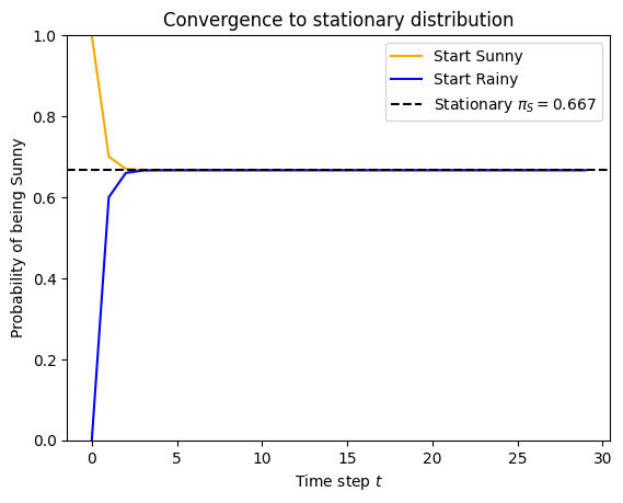
\pi_S = \frac{0.6}{0.9} \approx 0.667, \qquad \pi_R = \frac{0.3}{0.9} \approx 0.333.

(A3.8)

This means that in the long run, approximately 2 out of every 3 days are sunny, regardless of the weather on the first day.

Example: Verifying Ergodicity and Computing the Stationary Distribution¶

Consider the $3 \times 3$ transition matrix:

P = \begin{pmatrix} 0 & 0.6 & 0.4 \\ 0.3 & 0 & 0.7 \\ 0.5 & 0.5 & 0 \end{pmatrix}

(A3.9)

Step 1: Check irreducibility. Inspect $P$ and $P^2$ :

P^2 = P \cdot P = \begin{pmatrix} 0.38 & 0.20 & 0.42 \\ 0.35 & 0.53 & 0.12 \\ 0.15 & 0.30 & 0.55 \end{pmatrix}

(A3.10)

All entries of $P^2$ are positive, confirming that every state can reach every other in at most 2 steps. The chain is irreducible.

Step 2: Check aperiodicity. Since $P^2$ has strictly positive diagonal entries ( $d_i = 1$ for all $i$ ), the chain is aperiodic.

Step 3: Solve $\pi P = \pi$ . We solve:

\begin{align*} \begin{pmatrix} \pi_1 & \pi_2 & \pi_3 \end{pmatrix} \begin{pmatrix} 0 & 0.6 & 0.4 \\ 0.3 & 0 & 0.7 \\ 0.5 & 0.5 & 0 \end{pmatrix} \\ &= \begin{pmatrix} \pi_1 & \pi_2 & \pi_3 \end{pmatrix} \end{align*}

(A3.11)

This gives:

0.3\pi_2 + 0.5\pi_3 = \pi_1, \quad 0.6\pi_1 + 0.5\pi_3 = \pi_2, \quad 0.4\pi_1 + 0.7\pi_2 = \pi_3

(A3.12)

Replace the third equation with $\pi_1 + \pi_2 + \pi_3 = 1$ and solve to obtain:

\pi = \left(\frac{65}{227},\; \frac{80}{227},\; \frac{82}{227}\right) \approx (0.286,\; 0.352,\; 0.361).

(A3.13)

Exercises¶

Programming¶

Computing the Stationary Distribution with NumPy¶

The stationary distribution $\pi$ satisfies $\pi P = \pi$ , which is equivalent to $\pi (P - I) = 0$ . To compute it numerically, we replace one equation with the normalisation constraint $\sum_i \pi_i = 1$ :

import numpy as np

def stationary_distribution(P):
    """Compute the stationary distribution of an ergodic transition matrix."""
    n = P.shape[0]
    A = (P - np.eye(n)).T
    # Replace last row with normalisation constraint
    A[-1, :] = 1.0
    b = np.zeros(n)
    b[-1] = 1.0
    return np.linalg.solve(A, b)

# Weather example
P_weather = np.array([[0.7, 0.3],
                       [0.6, 0.4]])

pi = stationary_distribution(P_weather)
print(f"Stationary distribution: Sunny={pi[0]:.4f}, Rainy={pi[1]:.4f}")

Stationary distribution: Sunny=0.6667, Rainy=0.3333

Verifying Convergence¶

We can verify the Ergodic Theorem numerically by powering the transition matrix:

# Confirm convergence: P^t rows all approach pi as t grows large
P_power = np.linalg.matrix_power(P_weather, 50)
print("P^50 (rows should all equal stationary distribution):")
print(np.round(P_power, 6))

P^50 (rows should all equal stationary distribution):
[[0.666667 0.333333]
 [0.666667 0.333333]]

Stationary Distribution of a 3-State Chain¶

P_3 = np.array([[0.0, 0.6, 0.4],
                 [0.3, 0.0, 0.7],
                 [0.5, 0.5, 0.0]])

pi_3 = stationary_distribution(P_3)
print(f"Stationary distribution: {np.round(pi_3, 4)}")

# Verify: pi @ P should equal pi
print(f"Verification pi @ P: {np.round(pi_3 @ P_3, 4)}")

Stationary distribution: [0.2863 0.3524 0.3612]
Verification pi @ P: [0.2863 0.3524 0.3612]

Visualising Convergence from Different Starting States¶

import matplotlib.pyplot as plt

T = 30
pi_0_sunny = np.array([1.0, 0.0])  # start Sunny
pi_0_rainy = np.array([0.0, 1.0])  # start Rainy

dist_sunny = [pi_0_sunny @ np.linalg.matrix_power(P_weather, t) for t in range(T)]
dist_rainy = [pi_0_rainy @ np.linalg.matrix_power(P_weather, t) for t in range(T)]

plt.figure()
plt.plot([d[0] for d in dist_sunny], label="Start Sunny", color="orange")
plt.plot([d[0] for d in dist_rainy], label="Start Rainy", color="blue")
plt.axhline(pi[0], color="black", linestyle="--", label=f"Stationary $\\pi_S={pi[0]:.3f}$")
plt.xlabel("Time step $t$")
plt.ylabel("Probability of being Sunny")
plt.title("Convergence to stationary distribution")
plt.legend()
plt.ylim(0, 1);

Notable Research¶

The theory of ergodic Markov chains builds on the foundational work of Andrei Markov himself, who first studied the long-run behaviour of dependent random sequences in the early twentieth century.

The modern treatment of ergodic chains and stationary distributions is presented in the classical reference Kemeny & Snell, 1976, which establishes the Ergodic Theorem in the finite-state setting and its connections to the fundamental matrix theory of absorbing chains.

The application of ergodic theory to repeated games and direct reciprocity is central to the analysis of reactive strategies in the Prisoner’s Dilemma, as explored in Direct Reciprocity. The computation of long-run payoffs from stationary distributions provides the mathematical foundation for Press and Dyson’s influential analysis of memory-one strategies Press & Dyson, 2012.

Conclusion¶

This appendix introduced ergodic Markov chains and the Ergodic Theorem, which guarantees convergence to a unique stationary distribution for chains that are irreducible and aperiodic. These tools are essential for analysing systems that cycle indefinitely rather than being absorbed.

The key concepts are summarised in Table A3.1.

Table A3.1:Summary of ergodic Markov chains

Concept	Description
Irreducible Chain	Every state is reachable from every other state
Aperiodic Chain	No state is locked into returning only at multiples of a fixed period
Ergodic Chain	Irreducible and aperiodic; converges to a unique stationary distribution
Stationary Distribution	$\pi P = \pi$ , $\sum \pi_i = 1$ ; gives long-run fraction of time in each state
Ergodic Theorem	$\pi^{(0)} P^t \to \pi$ for any initial distribution $\pi^{(0)}$

Solutions¶

Solution to Exercise A3.1 #

1. $P = \begin{pmatrix}0 & 1 \\ 1 & 0\end{pmatrix}$

Irreducible? Yes: from state 1 we reach state 2 in one step, and from state 2 we reach state 1 in one step.
Aperiodic? No. The period of each state is $d = 2$ , since return to state 1 is only possible in an even number of steps (2, 4, 6, ...). The diagonal of $P$ is zero, and $P^2 = I$ has positive diagonal, confirming period 2.
Ergodic? No (not aperiodic).

Since the chain is not ergodic, the Ergodic Theorem does not apply in its strong form. However, because the chain is irreducible, there is still a unique stationary distribution. Solving $\pi P = \pi$ with $\pi_1 + \pi_2 = 1$ gives $\pi_2 = \pi_1$ and hence $\pi = (1/2, 1/2)$ . The long-run time average is $(1/2, 1/2)$ , but the chain does not converge from an arbitrary starting point; it oscillates.

2. $P = \begin{pmatrix}0.5 & 0.5 \\ 0.3 & 0.7\end{pmatrix}$

Irreducible? Yes: both off-diagonal entries are positive.
Aperiodic? Yes: both diagonal entries are positive ( $P_{11} = 0.5 > 0$ and $P_{22} = 0.7 > 0$ ), so each state has a self-loop and $d_i = 1$ .
Ergodic? Yes.

Stationary distribution. Solving $\pi P = \pi$ :

0.5 \pi_1 + 0.3 \pi_2 = \pi_1 \implies 0.3 \pi_2 = 0.5 \pi_1 \implies \pi_1 = \frac{3}{5}\pi_2

(A3.14)

With $\pi_1 + \pi_2 = 1$ :

\frac{3}{5}\pi_2 + \pi_2 = 1 \implies \pi_2 = \frac{5}{8}, \quad \pi_1 = \frac{3}{8}.

(A3.15)

So $\pi = (3/8,\ 5/8) = (0.375,\ 0.625)$ .

3. $P = \begin{pmatrix}1 & 0 & 0 \\ 0 & 0.5 & 0.5 \\ 0 & 0.5 & 0.5\end{pmatrix}$

Irreducible? No. State 1 has $P_{11} = 1$ (it is absorbing). Once the chain is in state 1 it never reaches states 2 or 3. States 2 and 3 communicate with each other but not with state 1.
Aperiodic? State 1 is aperiodic (self-loop). States 2 and 3 have period 1 since $P^2$ has positive diagonal entries. But irreducibility fails, so the question of chain-level aperiodicity is moot.
Ergodic? No (not irreducible).

The chain has multiple closed communicating classes and is therefore not ergodic; there is no unique stationary distribution for any initial state.

import numpy as np

def stationary_distribution(P):
    n = P.shape[0]
    A = (P - np.eye(n)).T
    A[-1, :] = 1.0
    b = np.zeros(n)
    b[-1] = 1.0
    return np.linalg.solve(A, b)

P2 = np.array([[0.5, 0.5], [0.3, 0.7]])
pi2 = stationary_distribution(P2)
print("Chain 2 stationary distribution:", np.round(pi2, 6))
# Verify
print("Verification pi @ P:", np.round(pi2 @ P2, 6))

Chain 2 stationary distribution: [0.375 0.625]
Verification pi @ P: [0.375 0.625]

Solution to Exercise A3.2 #

Let $P = \begin{pmatrix}1-a & a \\ b & 1-b\end{pmatrix}$ with $0 < a, b < 1$ .

Ergodicity. Since $a > 0$ and $b > 0$ , both off-diagonal entries are positive: state 1 can reach state 2 in one step and vice versa, so the chain is irreducible. The diagonal entries satisfy $1 - a \in (0, 1)$ and $1 - b \in (0, 1)$ , so both states have self-loops and $d_i = 1$ for all $i$ : the chain is aperiodic. Hence it is ergodic for any $a, b \in (0, 1)$ .
Stationary distribution. The condition $\pi P = \pi$ gives:
$\pi_1(1 - a) + \pi_2 b = \pi_1 \implies \pi_1 a = \pi_2 b \implies \pi_1 = \frac{b}{a}\pi_2.$
(A3.16)
Using $\pi_1 + \pi_2 = 1$ :
$\frac{b}{a}\pi_2 + \pi_2 = 1 \implies \pi_2\frac{a + b}{a} = 1 \implies \pi_2 = \frac{a}{a + b}.$
(A3.17)
Therefore:
$\pi_1 = \frac{b}{a + b}, \qquad \pi_2 = \frac{a}{a + b}.$
(A3.18)
Condition for uniform stationary distribution. We need $\pi_1 = \pi_2 = 1/2$ :
$\frac{b}{a + b} = \frac{1}{2} \Leftrightarrow 2b = a + b \Leftrightarrow a = b.$
(A3.19)
The stationary distribution is uniform if and only if $a = b$ , the two transition rates are equal.

import sympy as sym

a, b = sym.symbols("a b", positive=True)
P_sym = sym.Matrix([[1 - a, a], [b, 1 - b]])

pi1, pi2 = sym.symbols("pi_1 pi_2")
eqs = [
    sym.Eq(pi1 * (1 - a) + pi2 * b, pi1),
    sym.Eq(pi1 + pi2, 1),
]
sol = sym.solve(eqs, [pi1, pi2])
print("Stationary distribution:")
print("pi_1 =", sol[pi1])
print("pi_2 =", sol[pi2])

Stationary distribution:
pi_1 = b/(a + b)
pi_2 = a/(a + b)

# Condition for pi_1 = pi_2
condition = sym.solve(sym.Eq(sol[pi1], sym.Rational(1, 2)), a)
print("Condition for uniform distribution: a =", condition)

Condition for uniform distribution: a = [b]

Solution to Exercise A3.3 #

The weather chain from Motivating Example: Long-Run Behaviour in a Cycling System has:

P = \begin{pmatrix}0.7 & 0.3 \\ 0.6 & 0.4\end{pmatrix}

(A3.20)

with $\alpha = 0.3$ , $\beta = 0.6$ and stationary distribution $\pi = (2/3, 1/3)$ .

Computing $\pi^{(1)}$ and $\pi^{(2)}$ from $\pi^{(0)} = (1, 0)$ .
$\begin{align*} \pi^{(1)} &= \pi^{(0)} P = (1, 0) \begin{pmatrix}0.7 & 0.3 \\ 0.6 & 0.4\end{pmatrix} \\ &= (0.7,\ 0.3). \end{align*}$
(A3.21)
$\begin{align*} \pi^{(2)} &= \pi^{(1)} P = (0.7, 0.3) \begin{pmatrix}0.7 & 0.3 \\ 0.6 & 0.4\end{pmatrix} \\ &= (0.7 \times 0.7 + 0.3 \times 0.6,\ 0.7 \times 0.3 + 0.3 \times 0.4) \\ &= (0.49 + 0.18,\ 0.21 + 0.12) \\ &= (0.67,\ 0.33). \end{align*}$
(A3.22)
Distance from the stationary distribution. The stationary distribution is $\pi = (2/3, 1/3) \approx (0.6\overline{6}, 0.3\overline{3})$ .
$\begin{align*} \|\pi^{(2)} - \pi\|_1 &= |0.67 - 0.6\overline{6}| + |0.33 - 0.3\overline{3}| \\ &= 0.003\overline{3} + 0.003\overline{3} \approx 0.0067. \end{align*}$
(A3.23)
After only two steps, the distribution is within less than 1% of the stationary distribution in $\ell^1$ distance. Convergence is very fast.
Eigenvalues of $P$ . The characteristic polynomial of $P$ is:
$\begin{align*} \det(P - \lambda I) &= (0.7 - \lambda)(0.4 - \lambda) - (0.3)(0.6) \\ &= \lambda^2 - 1.1\lambda + (0.28 - 0.18) \\ &= \lambda^2 - 1.1\lambda + 0.10. \end{align*}$
(A3.24)
The roots are:
$\begin{align*} \lambda &= \frac{1.1 \pm \sqrt{1.21 - 0.4}}{2} = \frac{1.1 \pm \sqrt{0.81}}{2} \\ &= \frac{1.1 \pm 0.9}{2}. \end{align*}$
(A3.25)
So $\lambda_1 = 1$ and $\lambda_2 = 0.1$ .
Verification: $|1 - \alpha - \beta| = |1 - 0.3 - 0.6| = |0.1| = 0.1 = |\lambda_2|$ . ✓
The second eigenvalue governs the exponential rate of convergence: $|\lambda_2|^t = 0.1^t$ , which decays rapidly (after just 2 steps, $|\lambda_2|^2 = 0.01$ ), consistent with the fast convergence observed above.

import numpy as np

P = np.array([[0.7, 0.3], [0.6, 0.4]])
pi_0 = np.array([1.0, 0.0])

pi_1 = pi_0 @ P
pi_2 = pi_1 @ P
print("pi^(1) =", pi_1)
print("pi^(2) =", pi_2)

pi_stationary = np.array([2/3, 1/3])
print("Stationary distribution:", np.round(pi_stationary, 6))
print("L1 distance after 2 steps:", np.sum(np.abs(pi_2 - pi_stationary)))

pi^(1) = [0.7 0.3]
pi^(2) = [0.67 0.33]
Stationary distribution: [0.666667 0.333333]
L1 distance after 2 steps: 0.006666666666666654

eigenvalues = np.linalg.eigvals(P)
print("Eigenvalues of P:", np.sort(eigenvalues)[::-1])
alpha, beta = 0.3, 0.6
print("|1 - alpha - beta| =", abs(1 - alpha - beta))

Eigenvalues of P: [1.  0.1]
|1 - alpha - beta| = 0.09999999999999998

Solution to Exercise A3.4 #

Two tit-for-tat (TFT) players with $(p, q) = (1, 0)$ each cooperate if the opponent cooperated last round and defect if the opponent defected last round. The four states are $\{CC, CD, DC, DD\}$ , where the first letter is player 1’s action and the second is player 2’s action in the previous round.

Transition matrix. Given current state (row player’s last action, column player’s last action):
- From $CC$ : TFT1 plays $C$ (since opponent played $C$ ; $p=1$ ) and TFT2 plays $C$ (since opponent played $C$ ; $p'=1$ ). Next state: $CC$ .
- From $CD$ : TFT1 plays $D$ (since opponent played $D$ ; $q=0$ ) and TFT2 plays $C$ (since opponent played $C$ ; $p'=1$ ). Next state: $DC$ .
- From $DC$ : TFT1 plays $C$ (since opponent played $C$ ; $p=1$ ) and TFT2 plays $D$ (since opponent played $D$ ; $q'=0$ ). Next state: $CD$ .
- From $DD$ : TFT1 plays $D$ (since opponent played $D$ ; $q=0$ ) and TFT2 plays $D$ (since opponent played $D$ ; $q'=0$ ). Next state: $DD$ .
The transition matrix (ordering states $CC, CD, DC, DD$ ) is:
$P = \begin{pmatrix} 1 & 0 & 0 & 0 \\ 0 & 0 & 1 & 0 \\ 0 & 1 & 0 & 0 \\ 0 & 0 & 0 & 1 \end{pmatrix}$
(A3.26)
Ergodicity. The chain is not ergodic:
- State $CC$ is absorbing ( $P_{CC,CC} = 1$ ). Once both cooperate, they cooperate forever.
- State $DD$ is absorbing ( $P_{DD,DD} = 1$ ). Once both defect, they defect forever.
- States $CD$ and $DC$ form a periodic communicating class with period 2 (they cycle: $CD \to DC \to CD \to \cdots$ ).
- The chain is reducible: state $CC$ cannot reach $DD$ or the $\{CD,DC\}$ cycle, and vice versa.
Therefore the chain is neither irreducible nor aperiodic, hence not ergodic.
Long-run distribution starting from $CC$ . Since $CC$ is an absorbing state and the game starts in $CC$ , the chain stays in $CC$ with probability 1 for all time. The long-run distribution is:
$\pi = (1, 0, 0, 0) \quad \text{(all probability in state } CC\text{)}.$
(A3.27)
In terms of the game: two TFT players who start by cooperating will cooperate forever. The long-run payoff per round equals the cooperation payoff $R$ .

import numpy as np

# TFT vs TFT transition matrix over states {CC, CD, DC, DD}
P_tft = np.array([
    [1, 0, 0, 0],  # CC -> CC
    [0, 0, 1, 0],  # CD -> DC
    [0, 1, 0, 0],  # DC -> CD
    [0, 0, 0, 1],  # DD -> DD
], dtype=float)

print("Transition matrix P:")
print(P_tft)

# Starting from CC (index 0), pi^(0) = (1, 0, 0, 0)
pi_0 = np.array([1.0, 0.0, 0.0, 0.0])
print("\nAfter 10 steps (from CC):", pi_0 @ np.linalg.matrix_power(P_tft, 10))

Transition matrix P:
[[1. 0. 0. 0.]
 [0. 0. 1. 0.]
 [0. 1. 0. 0.]
 [0. 0. 0. 1.]]

After 10 steps (from CC): [1. 0. 0. 0.]

References¶

Kemeny, J. G., & Snell, J. L. (1976). Finite Markov chains. Springer-Verlag.
Press, W. H., & Dyson, F. J. (2012). Iterated Prisoner’s Dilemma contains strategies that dominate any evolutionary opponent. Proceedings of the National Academy of Sciences, 109(26), 10409–10413.