The set of mixed strategies that best respond to some opponent strategy forms a polytope, and Nash equilibria correspond to complementary vertices of a pair of such polytopes. This chapter develops this geometric perspective and introduces the Lemke–Howson algorithm for finding Nash equilibria in two-player games.
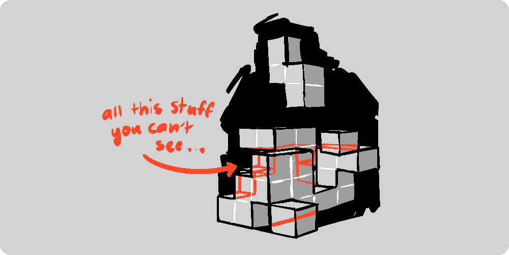
Figure 1:Geometric pieces fitting together. The best responses of each player form a polytope, and the Nash equilibria of a game sit at carefully matched vertices of a pair of such shapes.
Motivating Example: Insider Threat Detection
A large organization is conducting a red team exercise to test its internal security against potential insider threats.
A simulated Leaker (the row player) chooses among three methods of exfiltrating sensitive data: USB drive, Personal email, or Cloud storage.
The Defender (the column player) allocates monitoring resources to one of three detection strategies: Endpoint Monitoring, Email Filtering, or Cloud Auditing.
A government regulator observes the system and wants to assess whether current security measures are adequate. It is assumed that both players act optimally, i.e., they adopt strategies that correspond to a Nash equilibrium.
The regulator evaluates the system based on the equilibrium probability of a successful breach. If this exceeds a critical threshold, the regulator will mandate additional investment in security.
Let the row player (Leaker) choose among USB, Email, and Cloud, and let the column player (Defender) choose among Endpoint Monitoring, Email Filtering, and Cloud Auditing.
The Leaker’s payoff matrix (probabilities of successful exfiltration) is:
The Defender’s payoff matrix (probabilities of successful detection) is:
Note that the sum of payoffs in any outcome need not equal 1. This reflects the possibility that the attacker fails to exfiltrate and the defender fails to detect the attempt, for instance, if the file transfer crashes mid-way and no alert is triggered.
This point is also important mathematically: the game is not constant-sum and therefore not equivalent to a zero-sum game. It is also strategically rich: each player has three actions, none of which can be removed through simple rationalisation. This chapter introduces efficient methods for computing Nash equilibria in such settings.
Theory
Definition: Best Response Polytopes
For a two player game the row/column player best response polytope / is defined by:
The polytope , corresponds to the set of points with an upper bound on the utility of those points when considered as row strategies against which the column player plays.
The polytope , corresponds to the set of points with an upper bound on the utility of those points when considered as column strategies against which the row player plays.
Example: Best Response Polytopes for the threat detection game
Let us construct the best response polytopes for the threat detection game.
Applying the definition (3) we have:
This gives:
The vertices of these two polytopes are:
For :
These are shown in Figure 2.
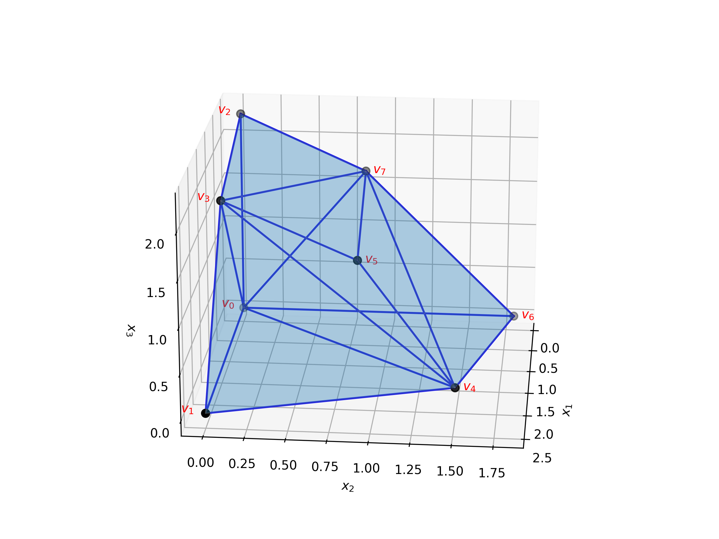
Figure 2:The three dimensional .
For :
These are shown in Figure 3.
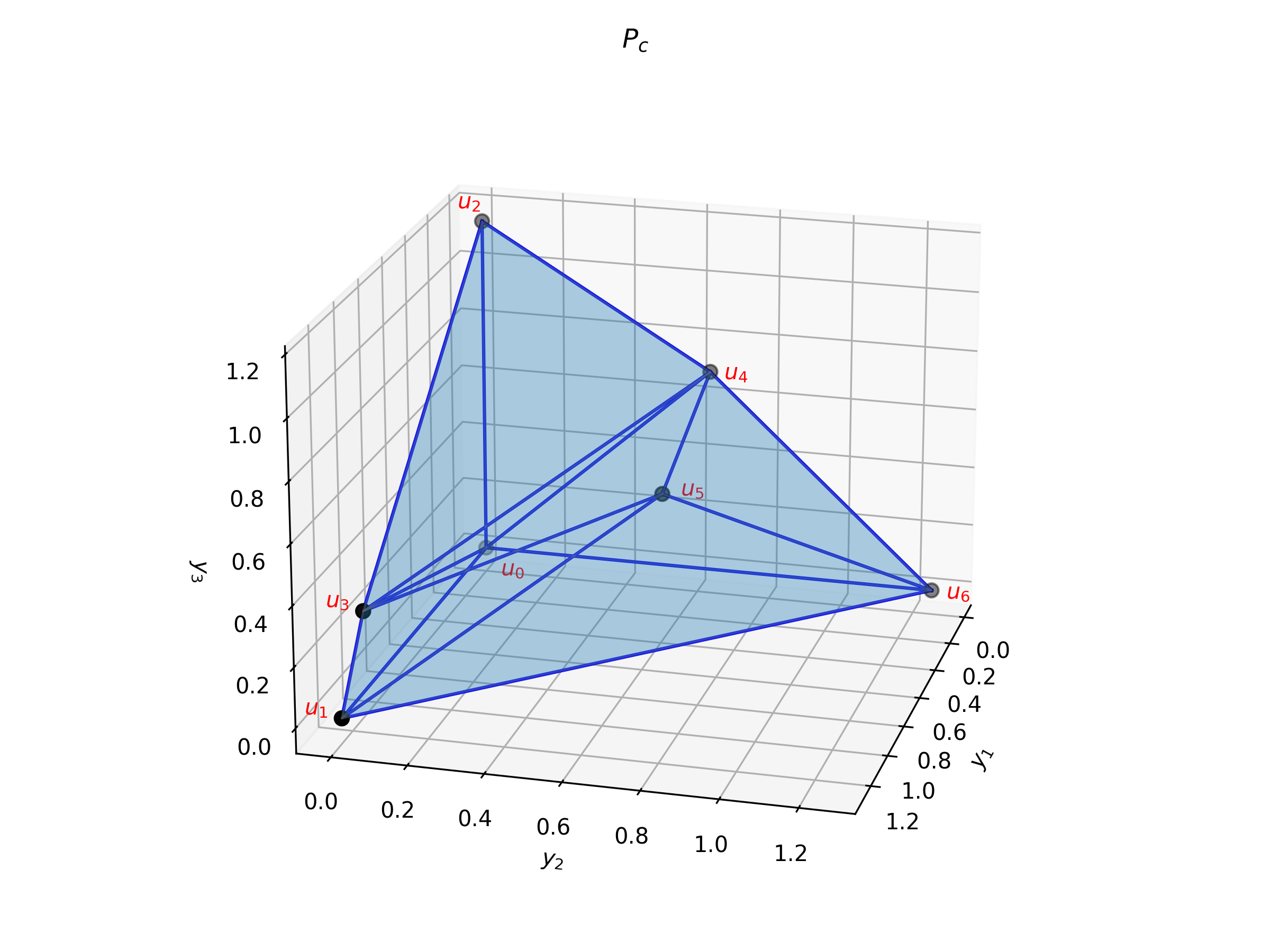
Figure 3:The three dimensional .
A vertex of a best response polytope corresponds to a strategy through normalization that ensures the sum corresponds to one.
For example corresponds to a strategy:
Similarly for :
Definition: Vertex Labelling
A vertex labelling is an assignment of labels to each vertex of a best response polytope, where each label corresponds to a constraint that is binding (i.e., holds with equality) at that vertex.
Each defining inequality of a best response polytope has a game theoretic interpretation when it is a binding inequality for a given vertex.
Example: Vertex labelling for the threat detection game
Let us consider the inequalities of and interpret what is implied when the inequality is binding:
Similarly for
We have used through as the labels.
Let us label each of the vertices:
For :
For :
For :
If a label is present in either vertex then either of the following are true:
it is indicating that an action is not played (for example label 1 in ).
it is indicating that the same action is a best response to the strategy represented by the vector (for example label 1 in ).
Looking at and the union of the labels of these vertices gives the full set of vertices.
This leads to the following definition.
Definition: Fully labelled vertex pair
A pair of vertices is said to be a fully labelled vertex pair if the union of their labels covers all possible labels:
Such a pair, when normalised (so that the components sum to 1), corresponds to a Nash equilibrium.
Example: Fully labelled vertex pair for the threat detection game
As shown in Example: Vertex labelling for the threat detection game:
is a fully labelled vertex pair.
This corresponds to the normalised strategies:
and
which is a Nash equilibrium.
Searching through all pairs of vertices is one approach to identifying Nash equilibria although a more efficient approach will now be discussed.
Definition: Lemke-Howson Algorithm
For a nondegenerate 2 player game the following algorithm returns a Nash equilibrium:
Start at the artificial equilibrium:
Choose a label to drop.
Remove this label from the corresponding vertex by traversing an edge of the corresponding polytope to another vertex.
The new vertex will now have a duplicate label in the other polytope. Remove this label from the vertex of the other polytope and traverse an edge of that polytope to another vertex.
Repeat step 4 until the pair of vertices is fully labelled.
Example: Application of the Lemke–Howson algorithm for the threat detection game with known vertices and labels
We will use Figure 2,
Figure 3, as well as
(16) and (17) to move
from vertex to vertex in the threat detection game.
We apply the algorithm as follows:
Start at and choose to drop label 1 (an arbitrary choice).
Label 1 is not among the labels of , so we move from to an adjacent vertex (, , , , , or ) that does not carry label 1 but shares other labels with . We select . This introduces label 6, which must now be dropped in .
: the labels are . Label 2 must be dropped in .
: the labels are . Label 5 must be dropped in .
: the labels are . Label 3 must be dropped in .
: the labels are . Label 4 must be dropped in .
: the labels are . This is a fully labelled vertex pair.
After normalisation, this yields the Nash equilibrium computed in
Example: Fully labelled vertex pair for the threat detection game.
This approach, while systematic, is only efficient here because the vertices
have already been computed. In practice, obtaining the vertices of the polytope
can be a time-consuming process. In the next example, we will demonstrate how
the Lemke–Howson algorithm becomes truly efficient through
integer pivoting.
Example: Application of the Lemke-Howson Algorithm for the threat detection game with integer pivoting
Using the definition of a tableau the tableaux for a 2 player game are given by:
and
In the case of the threat detection game this gives:
and
Let us now reproduce the steps of Example: Application of the Lemke–Howson algorithm for the threat detection game with known vertices and labels: we begin by dropping label 1 which corresponds to the non basic variable 1 of . In terms of integer pivoting this is done by pivoting the first column of .
As described in Definition: Integer Pivoting we carry out the minimum ratio test:
The ratio for the first row:
The ratio for the second row:
The ratio for the third row:
We pivot on the third row giving:
This tableau has labels/non basic variables . So we now pivot column 6 in . The minimum ratio test:
The ratio for the first row:
The ratio for the second row:
The ratio for the third row:
We pivot on the second row giving:
This tableau has labels so we pivot column 2 in . The minimum ratio test:
The ratio for the first row:
The ratio for the second row:
The ratio for the third row:
We pivot on the second row giving:
This tableau has labels so we pivot column 5 in . The minimum ratio test:
The ratio for the first row:
The ratio for the second row:
The ratio for the third row:
We pivot on the third row giving:
This tableau has labels so we pivot column 3 in . The minimum ratio test:
The ratio for the first row:
The ratio for the second row:
The ratio for the third row:
We pivot on the first row giving:
This tableau has labels so we pivot column 4 in . The minimum ratio test:
The ratio for the first row:
The ratio for the second row:
The ratio for the third row:
We pivot on the first row giving:
This tableau has labels so we have a fully labelled vertex pair.
Setting the non-basic variables to 0 we have the following systems of equations:
and:
Giving: and which when normalised (20) - (21) gives:
Exercises
Programming
Vertex enumeration with Nashpy
Nashpy can be used to generate the polytopes and enumerate all pairs of vertices.
import nashpy as nash
import numpy as np


M_r = np.array([
    [3, 1, 2],
    [2, 4, 1],
    [1, 3, 0]
])

M_c = np.array([
    [2, 3, 1],
    [1, 2, 4],
    [5, 1, 3]
])

game = nash.Game(M_r, M_c)
print(list(game.vertex_enumeration()))
[(array([0.5, 0.5, 0. ]), array([-2.42861287e-17, 2.50000000e-01, 7.50000000e-01]))]
Lemke-Howson with Nashpy
Nashpy can be used to carry out the Lemke-Howson algorithm, an efficient way to find a Nash equilibrium.
label_to_drop = 0
print(f"Nash equilibrium: {game.lemke_howson(initial_dropped_label=label_to_drop)}")
Nash equilibrium: (array([0.5, 0.5, 0. ]), array([0. , 0.25, 0.75]))
You can also enumerate all possible dropped labels:
print(list(game.lemke_howson_enumeration()))[(array([0.5, 0.5, 0. ]), array([0. , 0.25, 0.75])), (array([0.5, 0.5, 0. ]), array([0. , 0.25, 0.75])), (array([0.5, 0.5, 0. ]), array([0. , 0.25, 0.75])), (array([0.5, 0.5, 0. ]), array([0. , 0.25, 0.75])), (array([0.5, 0.5, 0. ]), array([0. , 0.25, 0.75])), (array([0.5, 0.5, 0. ]), array([0. , 0.25, 0.75]))]
Vertex enumeration with Gambit
Gambit can be used to enumerate all pairs of vertices:
import pygambit as gbt

game = gbt.Game.from_arrays(M_r, M_c)
print(gbt.nash.enummixed_solve(game))
NashComputationResult(method='enummixed', rational=True, use_strategic=True, equilibria=[[[Rational(1, 2), Rational(1, 2), Rational(0, 1)], [Rational(0, 1), Rational(1, 4), Rational(3, 4)]]], parameters={})
Lemke-Howson with Gambit
Gambit can be used to carry out the Lemke-Howson algorithm:
print(gbt.nash.lcp_solve(game))NashComputationResult(method='lcp', rational=True, use_strategic=True, equilibria=[[[Rational(1, 2), Rational(1, 2), Rational(0, 1)], [Rational(0, 1), Rational(1, 4), Rational(3, 4)]]], parameters={'stop_after': None, 'max_depth': None})
Notable Research
The original paper presenting the Lemke–Howson algorithm for two-player games is Lemke & Howson, 1964. That paper also contains a constructive proof that, in nondegenerate games, the number of Nash equilibria is always Exercise 4. The algorithm was later extended to -player games in Wilson, 1971, where the oddness result is also generalised. An alternative proof of the oddness theorem is provided in Harsanyi, 1973 the author of which was awarded the Nobel prize with Nash and Selten in 1994.
The worst-case complexity of the Lemke–Howson algorithm is analysed in Savani & Von Stengel, 2004, which demonstrates that the algorithm may require exponential time on specific inputs. Computing Nash equilibria is a computationally challenging task; this intuitive difficulty is formalised in @chen2006settling, Daskalakis et al., 2009, where the problem is shown to be PPAD-complete, placing it in a class of problems believed not to admit polynomial-time solutions.
Conclusion
This chapter introduced the geometric and algorithmic structure underlying Nash equilibrium computation through the lens of best response polytopes. By framing strategy sets as polytopes and interpreting labels as binding constraints, we gain powerful visual and computational tools for equilibrium analysis.
The Lemke–Howson algorithm provides a systematic method for tracing paths through these polytopes to identify fully labelled vertex pairs, which correspond to Nash equilibria. Though simple in low dimensions, this method scales to more complex games using tableau-based pivoting techniques such as integer pivoting.
Understanding the polyhedral structure of best responses not only aids in computational efficiency but also provides conceptual clarity: each equilibrium arises from a delicate balance of incentives, visible in the geometry of the feasible region.
Table 1 summarises the key concepts introduced in this chapter.
Table 1:Summary of best response polytopes
| Concept | Description |
|---|---|
| Best response polytope | A polyhedron defined by inequalities corresponding to best response conditions. |
| Binding inequality | A constraint that holds with equality at a vertex; gives rise to a label. |
| Vertex labelling | A mapping from vertices to labels indicating inactive actions or best responses. |
| Fully labelled vertex pair | A pair of vertices whose labels cover all actions, corresponds to a Nash equilibrium. |
| Lemke–Howson algorithm | A path-following method that constructs equilibria by dropping and replacing labels. |
| Integer pivoting | A tableau-based pivoting method used to trace Lemke–Howson paths efficiently. |
Solutions
- Lemke, C. E., & Howson, J. T., Jr. (1964). Equilibrium points of bimatrix games. Journal of the Society for Industrial and Applied Mathematics, 12(2), 413–423.
- Wilson, R. (1971). Computing equilibria of n-person games. SIAM Journal on Applied Mathematics, 21(1), 80–87.
- Harsanyi, J. C. (1973). Oddness of the number of equilibrium points: a new proof. International Journal of Game Theory, 2(1), 235–250.
- Savani, R., & Von Stengel, B. (2004). Exponentially many steps for finding a Nash equilibrium in a bimatrix game. 45th Annual IEEE Symposium on Foundations of Computer Science, 258–267.
- Daskalakis, C., Goldberg, P. W., & Papadimitriou, C. H. (2009). The complexity of computing a Nash equilibrium. Communications of the ACM, 52(2), 89–97.