Sustained cooperation over time depends on players remembering past interactions
and responding to them appropriately. This chapter begins with Axelrod’s
computer tournaments, which identified strategies that succeed in the iterated
Prisoner’s Dilemma, before focusing on reactive strategies: a tractable class
that conditions only on the opponent’s last move.
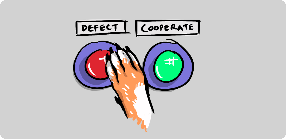
Figure 1:Cooperate or defect: in a repeated encounter each player presses one button at
a time, with an eye on how the other has played before. Direct reciprocity
studies how such conditional responses sustain cooperation.
Alice and Bob are researchers who meet regularly to share results before
submitting papers. At each meeting, each can choose to:
Cooperate (C): share their latest findings openly.
Defect (D): withhold key results to protect their competitive advantage.
The payoff structure is that of a Prisoner’s Dilemma: mutual sharing is
best collectively, but each individual has a short-term incentive to withhold.
The Folk Theorem tells us that cooperation can be
sustained in an infinitely repeated game: but it does not say how.
In practice, Alice and Bob remember only the last meeting. Alice might decide:
“I’ll share if you shared last time, but withhold if you withheld.” This
memory-one approach, conditioning solely on the previous round’s outcome,
is both cognitively realistic and mathematically tractable.
This chapter asks: which reactive strategies actually sustain cooperation,
and what are their long-run payoffs?
We start by giving a more general definition of Example: Prisoners’ Dilemma.
This game captures the fundamental structure of direct reciprocity in a repeated
game setting.
This requires 1+μ>1 and 0>−μ, both of which hold for μ>0.
The constraint 2R>T+S gives 2>1, which always holds.
This parametrisation is convenient: μ>0 is the only condition needed.
In 1980, Robert Axelrod organised a computer tournament for the iterated
Prisoner’s Dilemma Axelrod, 1980.
Fourteen strategies were submitted.
The tournament was a round-robin of 200 iterations, plus a strategy playing
uniformly at random.
Some entries were highly sophisticated; one used a χ2 test to detect
random opponents.
The winner was the simplest entry: Tit For Tat (TFT), which cooperates
on the first move then copies the opponent’s previous action.
A second tournament with 62 submissions followed Axelrod, 1980. With
participants now aware of TFT’s success, many strategies were designed
specifically to counter it. TFT won again.
These results suggested four principles for successful cooperation:
Don’t be envious: don’t strive for a higher score than your opponent.
Be nice: never defect first.
Reciprocate: match cooperation with cooperation, defection with defection.
Don’t be too clever: avoid overly complex exploitation.
Cooperates with probability 1/2 regardless of context
Generous Reciprocator
(0.9,0.3)
Strongly reciprocates cooperation; sometimes forgives
Suspicious Reciprocator
(0.7,0.1)
Cautiously cooperative; rarely forgives defection
Definition: Markov Chain of Two Reactive Strategies
When players with reactive strategies (p,q) and (p′,q′) play an
infinitely repeated Prisoner’s Dilemma, the pair of actions at each round
defines a Markov chain with state space
S={CC,CD,DC,DD}.
The transition matrix P∈R4×4, with rows and columns
ordered as (CC,CD,DC,DD), is:
where rows correspond to the current state and columns to the next state.
The entry Mss′ is the probability of transitioning from state s to
state s′. For example, from state CD (player 1 cooperated, player 2
defected): player 1 now cooperates with probability q (their opponent
defected), while player 2 now cooperates with probability p′ (their opponent
cooperated).
Theorem: Long-Run Average Payoffs via Stationary Distribution
If the Markov chain defined by (p,q) and (p′,q′) is ergodic (see
Appendix A3), it has a unique stationary
distribution π=(πCC,πCD,πDC,πDD) satisfying:
The values s1 and s2 are the long-run cooperation probabilities of each
player. The stationary distribution factorises as a product of marginals, so
the players’ long-run actions are independent despite their strategies being
correlated round-to-round.
Verify by direct substitution: set
π=(s1s2,s1(1−s2),(1−s1)s2,(1−s1)(1−s2)) and confirm
πM=π holds with the transition matrix from the definition above:
After carrying out the multiplication, each component of πM reduces to the
corresponding component of π when s1 and s2 satisfy the given
expressions. The algebra is routine but lengthy.
Example: Long-run payoffs for two reactive strategies
The Suspicious Reciprocator earns a higher long-run payoff. Despite cooperating
less, their lower generosity extracts value from the Generous Reciprocator’s
willingness to forgive defections.
Computing the Stationary Distribution of a Reactive Strategy Pair
Given the transition matrix P for two reactive strategies, the stationary
distribution satisfies πP=π. We can find it by solving the linear
system (PT−I)πT=0 subject to ∑πi=1.
import numpy as np

def reactive_transition_matrix(p, q, p_prime, q_prime):
    """
    Build the 4x4 transition matrix for reactive strategies (p,q) and (p',q').
    States are ordered: CC, CD, DC, DD.
    """
    M = np.array([
        [p * p_prime,       p * (1 - p_prime),       (1 - p) * p_prime,       (1 - p) * (1 - p_prime)],
        [q * p_prime,       q * (1 - p_prime),       (1 - q) * p_prime,       (1 - q) * (1 - p_prime)],
        [p * q_prime,       p * (1 - q_prime),       (1 - p) * q_prime,       (1 - p) * (1 - q_prime)],
        [q * q_prime,       q * (1 - q_prime),       (1 - q) * q_prime,       (1 - q) * (1 - q_prime)],
    ])
    return M

def stationary_distribution(M):
    """
    Compute the stationary distribution of a transition matrix M.
    """
    n = M.shape[0]
    A = (M.T - np.eye(n))
    A[-1, :] = 1
    b = np.zeros(n)
    b[-1] = 1
    return np.linalg.solve(A, b)

# Generous Reciprocator vs Suspicious Reciprocator
p, q = 0.9, 0.3
p_prime, q_prime = 0.7, 0.1

M = reactive_transition_matrix(p, q, p_prime, q_prime)
print("Transition matrix:")
print(np.round(M, 4))

pi = stationary_distribution(M)
print("\nStationary distribution (CC, CD, DC, DD):")
print(np.round(pi, 4))
# Compute long-run average payoffs
R, S, T, P = 3, 0, 5, 1

u1_bar = R * pi[0] + S * pi[1] + T * pi[2] + P * pi[3]
u2_bar = R * pi[0] + T * pi[1] + S * pi[2] + P * pi[3]

print(f"Long-run average payoff for Player 1: {u1_bar:.4f}")
print(f"Long-run average payoff for Player 2: {u2_bar:.4f}")
Long-run average payoff for Player 1: 1.9414
Long-run average payoff for Player 2: 2.5664
The axelrod Python library Knight et al., 2016 provides over 240 strategies
and tools to run reproducible tournaments, extending Axelrod’s original
experiments to much larger and more diverse strategic populations.
The Axelrod library provides axl.ReactivePlayer, which takes the reactive
strategy parameters (p,q) directly, matching the notation used throughout
this chapter.
The following code runs a long match between the Generous Reciprocator
(p,q)=(0.9,0.3) and the Suspicious Reciprocator (p′,q′)=(0.7,0.1)
from the example above
and compares the result to the closed-form payoffs.
import axelrod as axl
import numpy as np

generous = axl.ReactivePlayer(probabilities=(0.9, 0.3))
suspicious = axl.ReactivePlayer(probabilities=(0.7, 0.1))

match = axl.Match([generous, suspicious], turns=10000, seed=0)
match.play()
u1, u2 = match.final_score_per_turn()
print(f"Simulated:   Generous={u1:.4f}, Suspicious={u2:.4f}")
print(f"Theoretical: Generous={497/256:.4f}, Suspicious={657/256:.4f}")
/home/runner/work/gtb/gtb/.venv/lib/python3.14/site-packages/axelrod/strategies/zero_determinant.py:25: SyntaxWarning: "\m" is an invalid escape sequence. Such sequences will not work in the future. Did you mean "\\m"? A raw string is also an option.
  &s_{min} &= -\min\\left( \\frac{T - l}{l - S}, \\frac{l - S}{T - l}\\right) <= s <= 1
Reactive strategies are a subclass of memory-one strategies, which
condition on the full previous outcome (a1,a2)∈{C,D}2 rather than
just the opponent’s last action. The Axelrod library includes many built-in
memory-one strategies.
import axelrod as axl
import numpy as np

# Some notable memory-one strategies included in the library
players = [
    axl.TitForTat(),       # reactive: (p, q) = (1, 0)
    axl.ZDGTFT2(),         # generous zero-determinant strategy
    axl.ZDExtortion(),     # extortionate zero-determinant strategy
    axl.Cooperator(),      # reactive: (p, q) = (1, 1)
    axl.Defector(),        # reactive: (p, q) = (0, 0)
]

tournament = axl.Tournament(
    players=players, turns=200, repetitions=20, seed=0
)
results = tournament.play(progress_bar=False)
print("Ranking:")
for rank, name in enumerate(results.ranked_names):
    print(f"  {rank + 1}. {name}")
Ranking:
  1. Defector
  2. ZD-Extortion: 0.2, 0.1, 1
  3. Tit For Tat
  4. ZD-GTFT-2: 0.25, 0.5
  5. Cooperator
The Axelrod library documentation includes a tutorial showing how to replicate
Axelrod’s original 1980 tournament, providing a reproducible starting point for
exploring how strategy performance depends on the composition of the population.
The seminal empirical work on direct reciprocity is due to Robert Axelrod
Axelrod, 1980Axelrod, 1980, synthesised in his widely cited book
Axelrod, 1984. As described in Section 3,
Axelrod’s tournaments established Tit For Tat as the canonical cooperative
strategy and produced four heuristics for successful play.
Subsequent work has challenged these heuristics. The development of the Axelrod
Python library Knight et al., 2016 enabled systematic and reproducible analysis
across a far greater population of strategies. In particular,
Glynatsi et al., 2024 studied 45,600 tournaments across diverse strategic
populations and parameter regimes, finding that the original heuristics do not
generalise. The revised empirical findings suggest:
Be a little bit envious.
Be “nice” in non-noisy environments or when game lengths are longer.
Reciprocate both cooperation and defection appropriately.
It is acceptable to be clever.
Adapt to the environment.
The observation that being envious can be beneficial echoes a landmark
theoretical result. Press & Dyson, 2012 introduced zero-determinant
strategies, memory-one strategies that can unilaterally enforce linear payoff
relationships, including extortionate dynamics. This paper was described by
MIT Technology Review as having set “the world of game theory on fire.”
However, Hilbe et al., 2013 and Knight et al., 2018 showed that
extortionate strategies do not tend to survive under evolutionary dynamics,
tempering the initial excitement and reinforcing the importance of
adaptability.
This chapter examined how cooperation can emerge in pairwise repeated
interactions. Axelrod’s tournaments identified Tit For Tat as the canonical
cooperative strategy and produced four heuristics for successful play. These
heuristics have since been challenged: modern computational work, enabled by
large-scale reproducible tournaments, finds that what succeeds depends heavily
on the strategic population and game parameters.
The theoretical core of the chapter is the reactive strategy framework.
When two players use reactive strategies, their interaction defines a Markov
chain over outcome pairs, and the stationary distribution gives long-run
average payoffs. This connects the intuitions from Axelrod’s tournaments to a
rigorous mathematical foundation.
Axelrod, R. (1980). Effective choice in the prisoner’s dilemma. Journal of Conflict Resolution, 24(1), 3–25.
Axelrod, R. (1980). More effective choice in the prisoner’s dilemma. Journal of Conflict Resolution, 24(3), 379–403.
Knight, V. A., Campbell, O., Harper, M., Langner, K. M., Campbell, J., Campbell, T., Carney, A., Chorley, M., Davidson-Pilon, C., Glass, K., & others. (2016). An open framework for the reproducible study of the iterated prisoner’s dilemma. Journal of Open Research Software, 4(1).
Axelrod, R. (1984). The Evolution of Cooperation. Basic Books.
Glynatsi, N. E., Knight, V., & Harper, M. (2024). Properties of winning Iterated Prisoner’s Dilemma strategies. PLOS Computational Biology, 20(12), e1012644.
Press, W. H., & Dyson, F. J. (2012). Iterated Prisoner’s Dilemma contains strategies that dominate any evolutionary opponent. Proceedings of the National Academy of Sciences, 109(26), 10409–10413.
Hilbe, C., Nowak, M. A., & Sigmund, K. (2013). Evolution of extortion in iterated prisoner’s dilemma games. Proceedings of the National Academy of Sciences, 110(17), 6913–6918.
Knight, V., Harper, M., Glynatsi, N. E., & Campbell, O. (2018). Evolution reinforces cooperation with the emergence of self-recognition mechanisms: An empirical study of strategies in the Moran process for the iterated prisoner’s dilemma. PloS One, 13(10), e0204981.