The Biological Origins of Evolutionary Game Theory

Evolutionary biology poses questions that look surprisingly like strategic games: which traits persist in a population, and why? This chapter traces the biological origins of evolutionary game theory and motivates the dynamical models developed in the chapters that follow. It is intended as wider context rather than mathematical machinery: a reader following a purely mathematical path through the book can skip ahead to Replicator Dynamics without loss of continuity.

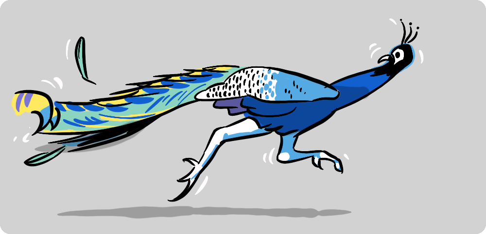
A peacock displaying its costly, extravagant tail. — Figure 1:A peacock’s tail is extravagant and costly to carry, yet it persists. Such apparently wasteful traits are a puzzle that evolutionary game theory helps to explain, much as it does the stag’s antlers in the example that follows.

Motivating Example: Why Don’t Stags Have Bigger Antlers?¶

Every autumn on the Scottish hillside, red deer stags compete for access to females. Stags with larger, heavier antlers are more likely to win contests Clutton-Brock et al., 1982Kruuk et al., 2002, but growing such antlers over the summer demands significant energy that could otherwise be allocated to body condition, immune function, and winter survival Moen et al., 1999Harshman & Zera, 2007.

Now consider the next few generations, as heavy antler growth spreads. Most stags now have large antlers. Contests between them are no longer quick or risk-free; both stags hold their ground, fights escalate, and serious injury becomes more likely. The energy diverted into growing large antlers no longer provides the same advantage it once did. A stag that allocates slightly less energy to antler growth may survive more winters, have more breeding opportunities, and ultimately achieve higher reproductive success than its heavily armed competitors Enquist & Leimar, 1987.

Thus, selection favours heavier antlers when they are rare, but this advantage diminishes as they become common. The fitness of any given antler size depends on what the rest of the population is doing: it is a game Maynard Smith & Price, 1973.

Why the stable antler size is not simply “as large as possible” cannot be answered by classical genetics alone; it requires the framework of evolutionary game theory, developed in this chapter.

Theory¶

Darwin’s Three Conditions¶

In 1859 Darwin proposed that the diversity of life could arise from a single, simple mechanism: no designer, no foresight, no goal. Three observable facts about populations are sufficient:

Variation. Individuals differ from one another in heritable traits: body size, beak shape, defensive behaviour.
Heritability. Offspring tend to resemble their parents more than they resemble randomly chosen members of the population. Traits are passed down.
Differential reproduction. Some individuals, by virtue of their traits, survive longer or leave more offspring than others.

When these three conditions hold, the composition of a population changes over time. Traits that help their bearers reproduce become more common in the next generation; traits that hinder reproduction fade away. Darwin called this process natural selection.

All three conditions hold for stag antlers. Antler size varies across individuals. It is partly inherited. And it affects how many offspring a stag leaves (via contest outcomes). Natural selection therefore acts on antler size; the only question is in which direction.

Genes, Loci, and Alleles¶

Darwin’s three conditions require heritable variation but say nothing about how inheritance works. The vocabulary of genetics makes the mechanism precise, and the same vocabulary maps cleanly onto the language of strategies.

A gene is a stretch of DNA that carries the instructions for some heritable feature. The fixed position a gene occupies on a chromosome is its locus, and the variant forms a gene can take at that locus are its alleles. Most animals are diploid: they carry two copies of each chromosome, and hence two alleles at every locus, one inherited from each parent. An individual carrying two copies of the same allele is homozygous at that locus; one carrying two different alleles is heterozygous.

When the two alleles differ, one is often dominant and masks the effect of the other, which is then recessive. Figure 2 shows a single locus with two alleles, the three diploid genotypes they produce, and the way those genotypes map to an observable feature when one allele is dominant.

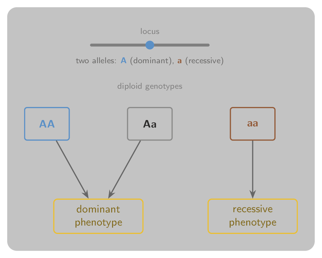
A single locus with two alleles A and a, the diploid genotypes AA, Aa and aa, and their mapping to dominant and recessive phenotypes. — Figure 2:A single locus carrying two alleles: the dominant A and the recessive a. The three diploid genotypes are AA, Aa, and aa. When A is dominant, both AA and Aa produce the dominant phenotype, and only aa produces the recessive one.

The central bookkeeping quantity of population genetics is the allele frequency: the proportion of all copies at a locus that are of a given allele. At its most basic, natural selection is change in allele frequency from one generation to the next. This is the biological counterpart of the strategy frequency $x$ that the later chapters track.

Genotype and Phenotype¶

The genotype of an organism is its inherited genetic constitution: the alleles it carries across all relevant loci. The genotype is fixed at conception and is what passes, one allele per locus, to each offspring.

The phenotype is the observable expression of that genotype in a given environment: the physical structure, physiological properties, and behavioural tendencies visible to natural selection. Antler size, plumage colour, and the propensity to escalate or retreat in a contest are all phenotypic traits.

The map from genotype to phenotype is rarely one-to-one. Most interesting traits are polygenic, shaped by many loci acting together, and the same genotype can yield different phenotypes in different environments. A stag well fed over the summer grows larger antlers than a genetically identical stag on poorer ground.

The crucial asymmetry is this: natural selection acts on phenotypes but changes the frequency of genotypes. A stag’s genotype specifies its antler-investment programme; the antlers that result are the phenotype; contest outcomes determine fitness; and fitness determines how many copies of the underlying genotype reach the next generation. Figure 3 shows the loop.

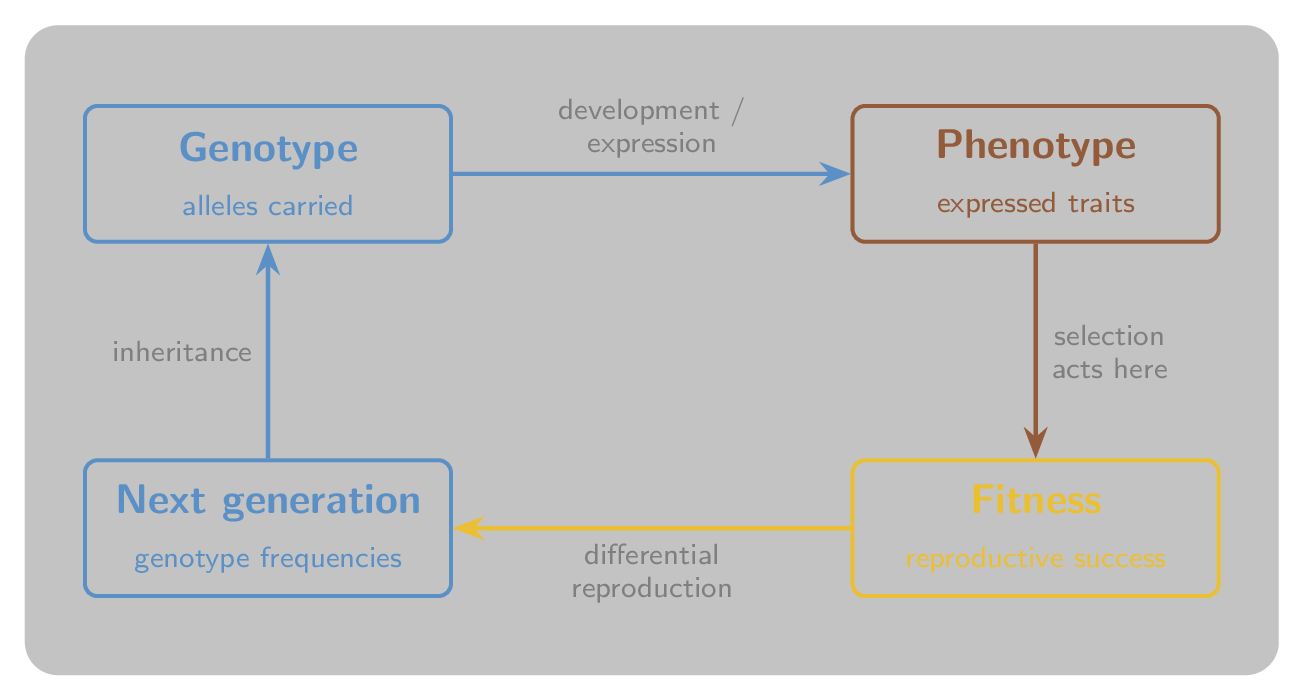
A cycle in which genotype develops into phenotype, selection acts on the phenotype to determine fitness, differential reproduction changes genotype frequencies in the next generation, and inheritance carries them forward. — Figure 3:The cycle of selection. The genotype develops into a phenotype; selection acts on the phenotype through reproductive success; differential reproduction changes the genotype frequencies in the next generation; and inheritance carries those genotypes forward. Selection reads the phenotype but rewrites the genotype frequencies.

The game-theoretic translation is direct: each distinct genotype (or allele at the relevant locus) corresponds to a strategy, and the phenotype is the strategy in action. What the replicator equation tracks over time is the frequency of genotypes, that is, of strategies, in the population.

Pleiotropy: One Gene, Many Traits¶

A single gene rarely affects just one trait. Pleiotropy is the phenomenon of one gene influencing several apparently unrelated phenotypic traits at once. Figure 4 illustrates the idea: a single allele feeds into more than one trait, so selection acting on one of those traits inevitably drags the others along with it.

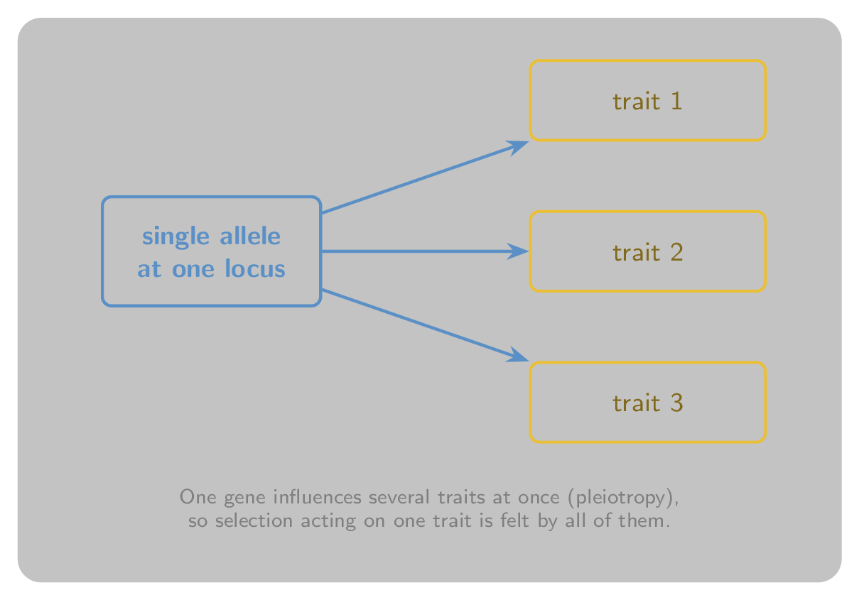
A single allele at one locus with arrows to three separate traits, illustrating pleiotropy. — Figure 4:Pleiotropy. A single allele at one locus influences several traits at once, so the traits cannot evolve independently of one another.

Pleiotropy matters here because it explains why a trait that lowers fitness on one axis need not be eliminated. An allele can be costly in one respect and beneficial in another, and selection acts on the net effect. This is a recurring theme: a strategy that looks individually disadvantageous can persist because of how it is tied to everything else going on in the population.

What Is a “Strategy” in Biology?¶

In game theory a strategy is a decision rule. In biology a strategy is an inherited behavioural tendency: the tendency to fight or retreat, to cooperate or defect, to invest heavily in display or conserve resources.

Biological strategies are not chosen. A stag does not calculate expected payoffs and decide on an antler investment level. It expresses a phenotype inherited from its parents. Individuals that happen to inherit strategies effective against the opponents they actually encounter leave more offspring. Those offspring inherit the same tendencies. Over generations, effective strategies spread.

The word “strategy” in evolutionary biology is shorthand for an inherited behavioural phenotype. The rational-agent interpretation is a useful fiction that lets us apply game-theoretic mathematics to a process that is entirely mechanical.

Fitness: Reproductive Success as Payoff¶

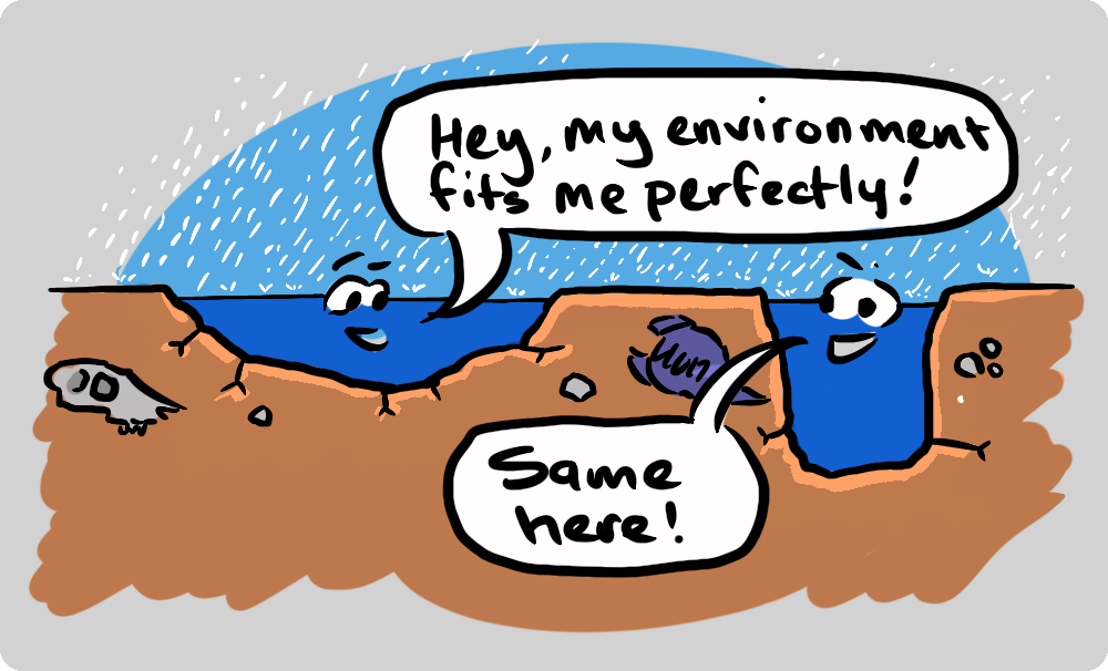
Two puddles, each remarking that their environment fits them perfectly. — Figure 5:“Survival of the fittest” is often misread as a contest, when it is really a statement of fit. A puddle is not in competition with the hole it sits in: it simply takes the shape that the hole allows. Fitness works the same way, it is not how strong or clever a type is in the abstract, but how well its traits match the environment it happens to occupy.

The central quantity in evolutionary biology is fitness, the expected number of surviving offspring an individual leaves. Variants with higher fitness leave more copies of themselves and so increase in frequency; variants with lower fitness decline. Fitness is the biological counterpart of a payoff: it is the currency in which natural selection keeps score.

In classical population genetics, fitness is treated as a fixed property of a type, a constant attached to each genotype regardless of how common it is. A type with above-average fitness then grows in frequency, generation on generation, until it dominates the population.

The stag example does not fit this picture. The advantage of heavy antler investment is large when such investment is rare and small when it is common, so fitness is not a fixed constant: it depends on the current composition of the population. Making that dependence precise is the subject of the next section, and turning it into a dynamical equation is the work of Replicator Dynamics.

Frequency-Dependent Selection¶

A hedgehog and a crab cooperating across species. — Figure 6:Cooperation between very different creatures. Whether such behaviour pays off depends on how common it is in the population, an idea made precise by frequency-dependent selection.

Selection is frequency-dependent when the fitness of a type depends on the current composition of the population, not just on its own properties in isolation.

Frequency dependence arises whenever individuals interact, which is essentially always in real populations. The stag antler example is a canonical instance, but the phenomenon is ubiquitous:

A bacterium that secretes a costly public-good molecule benefits the group but is exploited by non-secretors. Its fitness advantage depends on how many non-secretors are present.
A fish that mimics a toxic species is protected by predators, but only while the toxic species remains common enough for predators to have learned the association.
A worker bee that reproduces rather than works gains personally in the short run, but a colony of non-workers produces nothing and dies.

In all these cases, what makes a strategy “good” depends on what the rest of the population is doing.

A classical example of frequency-dependent selection predates Maynard Smith and Price by decades. Fisher’s argument for the 1:1 sex ratio Fisher, 1930 is a frequency-dependent argument in disguise: if either sex becomes rare, the per-capita reproductive success of producing offspring of that sex rises, so parents who invest in the rarer sex leave more grandchildren. The stable investment ratio is the one at which neither sex offers an advantage. This is the same balance condition that determines $x^*$ in Hawk–Dove and, more broadly, every mixed equilibrium we meet in the chapters that follow.

The Hawk–Dove Game¶

The stag example is formalised by the Hawk–Dove game, introduced by Maynard Smith and Price Maynard Smith & Price, 1973 to explain why animal contests so rarely escalate to serious injury.

Two strategies:

Hawk (H): always escalate; fight until injured or opponent retreats.
Dove (D): display first; retreat immediately if opponent escalates.

Each contest is over a resource worth $V > 0$ to the winner. A fight between two Hawks injures one of them at cost $C$ , where $C > V$ . The expected payoffs for each encounter type are:

\begin{array}{c|cc} & \text{meets H} & \text{meets D} \\ \text{H plays} & \frac{V-C}{2} & V \\ \text{D plays} & 0 & \frac{V}{2} \end{array}

(1)

Each strategy’s expected fitness depends on how common Hawks are. Writing $x$ for the fraction of Hawks, a Hawk does worse as $x$ rises, since it more often meets another Hawk and risks a costly fight, while a Dove does best when Hawks are rare. The two fitnesses are equal at a single interior frequency,

x^* = \frac{V}{C},

(2)

which lies strictly between 0 and 1 because $C > V$ . The stable outcome is therefore a mixed population, not fixation of either pure strategy: when Hawks are rarer than $x^*$ they do better and spread, and when they are commoner they do worse and decline, so the population is driven back to $x^*$ from either side, as Figure 7 shows. This balance point is a Nash equilibrium of the underlying game. The fitnesses are derived in full, and the sense in which $x^*$ is evolutionarily stable is made precise, in Replicator Dynamics.

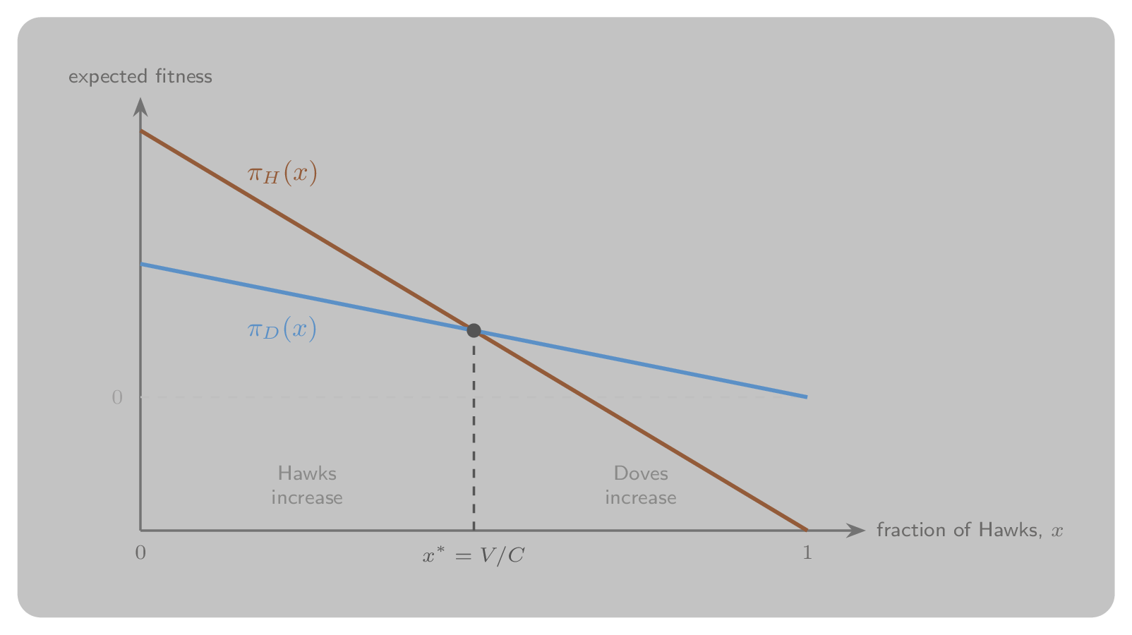
Expected fitness of Hawk and Dove as functions of the Hawk frequency x, two downward-sloping lines crossing at x* equals V over C. — Figure 7:Frequency-dependent fitness in the Hawk–Dove game. Each line gives the expected fitness of a strategy as the fraction of Hawks $x$ varies. The lines cross at $x^{*}=V/C$ : to the left of $x^{*}$ Hawks earn more and increase in frequency, to the right Doves earn more and Hawks decline. The population is driven back to $x^{*}$ from either side.

Two biological terms are worth noting at this point. A population is monomorphic if every individual plays the same strategy, and polymorphic if more than one strategy is present. The Hawk–Dove equilibrium admits both readings: as a polymorphic population in which a fraction $V/C$ of individuals are pure Hawks and the rest pure Doves, or as a monomorphic population in which every individual plays the mixed strategy $\sigma^* = (V/C,\, 1 - V/C)$ . The two readings give the same expected payoffs in a well-mixed population, and the mathematical chapters that follow treat them interchangeably.

Evolutionary stability¶

The Hawk–Dove game shows that neither pure Hawk nor pure Dove takes over: at $x^* = V/C$ each type has the same expected fitness. A sharper question is whether this composition is itself stable against the entry of novel behaviour. If a rare mutant playing a different strategy appeared, would selection eliminate it, or would it spread?

The mixed composition at $x^*$ has the property that residents always do strictly better than any rare mutant, so the mutant fades and the population returns to $x^*$ . Strategies with this property are called evolutionarily stable, a notion introduced by Maynard Smith and Price Maynard Smith & Price, 1973. For the Hawk–Dove game with $V < C$ , neither pure Hawk nor pure Dove is evolutionarily stable, but the mixed composition $\sigma^* = (V/C,\, 1 - V/C)$ is. The formal definition and its algebraic characterisation are developed in Replicator Dynamics.

The Bridge: Fitness Is Payoff¶

The conceptual step from population genetics to evolutionary game theory requires a single substitution:

Replace the fixed fitness constants of classical genetics with payoffs that depend on what strategies you encounter.

In a pairwise interaction model, where each individual is paired at random with another drawn from the population, the expected fitness of an individual using strategy $i$ in a population where strategy $j$ has frequency $x_j$ is:

\pi_i(x) = \sum_j x_j \cdot M_{ij}

(3)

where $M_{ij}$ is the payoff to strategy $i$ when meeting strategy $j$ . The payoff matrix $M$ is the fitness matrix. Strategies with above-average fitness increase in frequency; strategies with below-average fitness decline.

Table 1:The correspondence between population genetics and evolutionary game theory

Population genetics	Evolutionary game theory
Genotype / allele	Strategy
Absolute fitness $W_i$	Expected payoff $\pi_i$
Fitness advantage over mean	$\pi_i - \bar\pi$ drives frequency change
Frequency-dependent fitness	Payoff matrix $M_{ij}$
Mutation rate $\mu$	Strategy exploration / trembling hand
Population size $N$	Governs how much chance matters vs selection
Genetic drift	Stochastic fluctuations in finite-population models
Evolutionarily stable strategy	Nash equilibrium that selection cannot destabilise

What the Following Chapters Formalise¶

A coral polyp, a simple organism living as part of a larger colony. — Figure 8:A single polyp is a simple creature, yet colonies of them build reefs. Much of what follows asks how the behaviour of many simple individuals aggregates into the dynamics of a whole population.

The replicator dynamics takes the limit of a very large, well-mixed population and asks how strategy frequencies change continuously over time. The answer is the replicator equation $\dot x_i = x_i(\pi_i - \bar\pi)$ , the continuous-time mathematical form of natural selection under frequency-dependent fitness.

The Moran process takes a small, finite population seriously. In a small population, chance matters: even a fitter strategy can be lost by bad luck before it spreads. The Moran process models one individual being copied at each time step, and the key question is the fixation probability, the chance that a single mutant takes over rather than dying out.

The learning and evolutionary dynamics chapter asks what happens when individuals update strategies by imitation, rational introspection, or best-response. These social-learning mechanisms produce the same large-population limit as biological evolution, but differ in important ways in small populations.

Together these chapters show that the replicator equation is the universal large-population limit of all plausible evolutionary and social-learning update rules, and that the Nash equilibria of the stage game are its rest points.

Exercises¶

Exercise 2

Return to the stag antler example from Motivating Example: Why Don’t Stags Have Bigger Antlers?.

Identify which of Darwin’s three conditions (variation, heritability, and differential reproduction) are present in the stag antler scenario. Give a one-sentence justification for each condition.
Suppose a genetic study reveals that antler-investment level is not heritable: each stag grows antlers to a size determined entirely by random developmental noise, regardless of its father’s investment level. Which of Darwin’s three conditions would fail? Would natural selection still act on antler investment? Explain.
The chapter distinguishes genotype, phenotype, and strategy. In the context of antler investment, identify what each of these terms refers to, and explain why natural selection acts on the phenotype but changes the frequency of genotypes.

Notable Research¶

The founding paper of evolutionary game theory is Maynard Smith & Price, 1973, which introduced the Hawk–Dove game and the concept of an evolutionarily stable strategy. It was simultaneously a contribution to theoretical biology and a demonstration that Nash equilibrium analysis could be applied to non-rational agents. Maynard Smith later developed the theory in full in his book Maynard Smith, 1982.

The 1973 paper built on George Price’s covariance equation Price, 1970, which gave a clean algebraic statement of selection, and ran in parallel with William Hamilton’s earlier game-theoretic treatment of sex ratios and local mate competition Hamilton, 1967. Taken together, this body of work transformed mid-twentieth-century evolutionary biology from a purely genetic optimisation framework into one in which strategic interaction plays the central role.

The mathematical link between ESS and the dynamic stability of the replicator equation was established by Taylor & Jonker, 1978. This paper showed that evolutionary stability (a static, game-theoretic concept) and asymptotic stability under selection dynamics (a dynamical systems concept) are, under broad conditions, equivalent, justifying the use of Nash equilibrium as a prediction for biological populations.

The broader programme connecting population genetics to game theory, and showing that many different biological update rules share the same large-population limit, is surveyed in Nowak, 2006, which provides extensive biological examples alongside the mathematical theory.

Conclusion¶

Natural selection is not rational deliberation, but it produces outcomes that look as though it is. The reason is that evolution is a kind of optimisation, but what it optimises is reproductive success against the current population, not a fixed objective. Whenever reproductive success depends on what strategies your neighbours use, you have a game. The payoff matrix of that game is the fitness matrix of the biological population.

The three conditions for natural selection (variation, heritability, differential reproduction) translate directly into the components of the mathematical models in the chapters that follow:

Variation: multiple strategies coexist in the population.
Heritability: offspring adopt the parent strategy.
Differential reproduction: strategies that do better than average increase in frequency.

The evolutionary chapters of this book can be read as the mathematical consequences of applying these three conditions to populations playing games.

Table 2 summarises the key concepts introduced in this chapter.

Table 2:Summary of biological foundations

Concept	Description	Connects to
Natural selection	Differential reproduction of heritable variants	All evolutionary chapters
Genotype	Inherited genetic specification; determines available strategies	Strategy type in EGT
Phenotype	Observable expression of genotype visible to selection	Strategy played
Allele	Variant form of a gene; distinct alleles correspond to distinct strategies	Strategy in EGT
Fitness $W_i$	Expected reproductive output of type $i$	Payoff $\pi_i$ in evolutionary game theory
Frequency-dependent selection	Fitness depends on population composition	Payoff matrix $M_{ij}$
Hawk–Dove game	Canonical model of animal conflict	Replicator dynamics, ESS
Evolutionarily stable strategy	Nash equilibrium robust to rare invasion	Stable fixed points of replicator dynamics

Solutions¶

Solution to Exercise 1 #

The cryptic frequency rises monotonically from $x_C = 0.2$ toward fixation, levelling off near $x_C = 1$ . With cryptic beetles always reproducing above the population average, their share grows in every generation, slowly at first while they are rare, then more rapidly, then slowing again as they approach fixation.
The roles reverse. Against a pale, open background it is now the conspicuous morph that blends in, so it has the higher fitness. Starting from $x_C = 0.2$ , the cryptic frequency falls toward zero and the conspicuous morph fixes.
There is no universally fitter type. The same colour is advantageous in one environment and deleterious in another; what selection optimises is reproductive success in the current environment, not a fixed objective. When the environment changes, the direction of selection can reverse.

Solution to Exercise 2 #

All three conditions are present in the stag antler scenario.
- Variation. Stags differ in their antler-investment level: some invest heavily in growth, others minimally.
- Heritability. The tendency to invest in antler growth is partly inherited; offspring resemble their fathers in investment level more than they resemble a randomly chosen stag.
- Differential reproduction. Stags with larger antlers win more contests, gain access to more females, and leave more offspring than stags with smaller antlers.
Without heritability the second condition fails. Natural selection requires that fitness differences translate into changes in the composition of the next generation. If antler investment is entirely random and non-heritable, a high-investing stag may leave more offspring but those offspring do not inherit the high-investment tendency. The trait cannot increase in frequency across generations, so natural selection cannot act on it.
The genotype is the inherited genetic programme that specifies a stag’s antler-investment level: the alleles at the relevant loci that are passed from parent to offspring. The phenotype is the actual antler size that results when that programme is expressed, the structure visible to predators and rival stags. The strategy in the game-theoretic sense is the inherited behavioural tendency itself (invest heavily vs. invest lightly), which corresponds to the genotype. Natural selection acts on the phenotype because contest outcomes depend on actual antler size, not on the underlying genetics. But it is the genotype that is copied into the next generation, so selection on the phenotype translates into a change in the frequency of genotypes in the population.

Solution to Exercise 3 #

The brown phenotype is produced by $BB$ and $By$ ; the yellow phenotype only by $yy$ . The genotypes $BB$ and $yy$ are homozygous (two copies of the same allele), and $By$ is heterozygous (one copy of each).
A brown-shelled snail can be heterozygous, $By$ : it shows the brown phenotype because $B$ is dominant, yet it still carries the recessive $y$ allele. If two $By$ snails breed, an offspring can inherit $y$ from each parent and so be $yy$ , which is yellow. The phenotype hides the underlying genotype, so the recessive allele persists, unseen, in heterozygotes.
This is pleiotropy: one gene influencing more than one trait. Because the brown allele affects both colour and thickness, any selection on shell colour automatically shifts the distribution of shell thickness as well. The two traits are tied together through the same allele and cannot respond to selection independently.

Solution to Exercise 4 #

Not frequency-dependent. The plant’s improved photosynthesis gives a fixed advantage regardless of what other plants are doing. Fitness here is a constant property of the genotype, not a function of the population composition.
Frequency-dependent. The protection conferred by mimicry depends on how common the toxic model species is in the population. When the model is rare, predators have not learned the association, and the mimic gains little benefit. The fitness of the mimicry strategy depends on the frequency of the toxic model in the broader community, rather than on a constant property of the mimic itself.
Frequency-dependent. The fitness advantage of the secreting bacterium depends on the population composition. When non-secretors are rare, the enzyme cost is borne by nearly everyone and provides little competitive advantage; when non-secretors are common, secretors are exploited but the enzyme still raises mean colony output. The key point is that the fitness of the secreting strategy changes with the frequency of non-secretors in the population, which is precisely what frequency dependence means.
Not frequency-dependent (under the stated assumption). If faster cheetahs always catch more prey independently of what other cheetahs do, fitness is a constant function of speed and does not depend on the population composition. In practice, cheetah speed might interact with prey evolution (an arms race), but the scenario as stated implies constant fitness.

References¶

Clutton-Brock, T. H., Guinness, F. E., & Albon, S. D. (1982). Red Deer: Behavior and Ecology of Two Sexes. University of Chicago Press.
Kruuk, L. E. B., Slate, J., Pemberton, J. M., Brotherstone, S., Guinness, F., & Clutton-Brock, T. (2002). Antler size in red deer: heritability and selection but no evolution. Evolution, 56(8), 1683–1695. 10.1111/j.0014-3820.2002.tb01480.x
Moen, R. A., Pastor, J., & Cohen, Y. (1999). Antler growth and extinction of Irish elk. Evolutionary Ecology Research, 1(2), 235–249. http://www.evolutionary-ecology.com/abstracts/v01/1026.html
Harshman, L. G., & Zera, A. J. (2007). The cost of reproduction: the devil in the details. Trends in Ecology & Evolution, 22(2), 80–86. 10.1016/j.tree.2006.10.008
Enquist, M., & Leimar, O. (1987). Evolution of fighting behaviour: the effect of variation in resource value. Journal of Theoretical Biology, 127(2), 187–205. 10.1016/S0022-5193(87)80130-3
Maynard Smith, J., & Price, G. R. (1973). The Logic of Animal Conflict. Nature, 246, 15–18. 10.1038/246015a0
Fisher, R. A. (1930). The Genetical Theory of Natural Selection. Clarendon Press.
Maynard Smith, J. (1982). Evolution and the Theory of Games. Cambridge University Press.
Price, G. R. (1970). Selection and covariance. Nature, 227, 520–521. 10.1038/227520a0
Hamilton, W. D. (1967). Extraordinary sex ratios. Science, 156(3774), 477–488. 10.1126/science.156.3774.477
Taylor, P. D., & Jonker, L. B. (1978). Evolutionary stable strategies and game dynamics. Mathematical Biosciences, 40(1–2), 145–156.
Nowak, M. A. (2006). Evolutionary Dynamics: Exploring the Equations of Life. Harvard University Press.