Motivating Example: Two Views of a Polytope
Consider the following set of points:
This set is a polytope, defined as the convex hull of a finite set of vertices:
A visualization is provided in Figure A5.1.
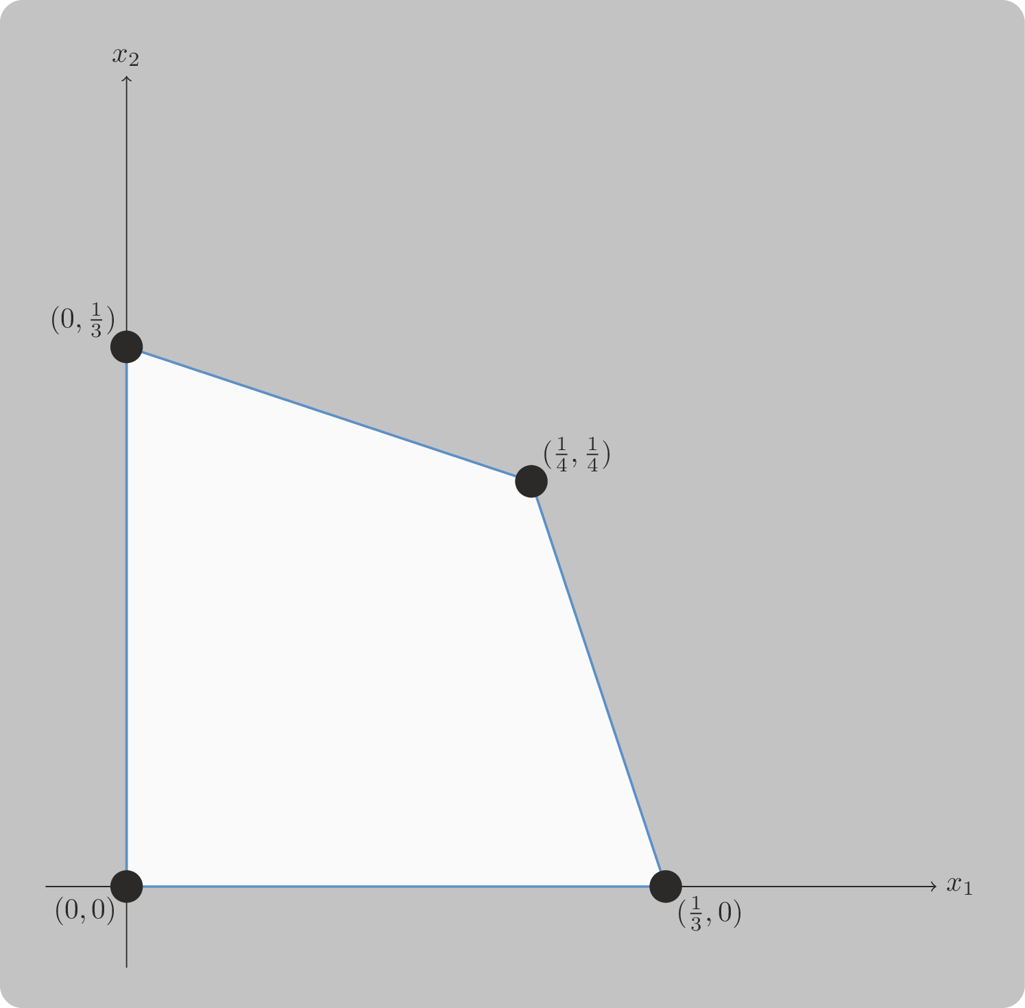
Figure A5.1:The two-dimensional polytope defined by (A5.1), shown as the convex hull of four points.
Polytopes can also be equivalently defined as the intersection of half- spaces, that is, bounded regions formed by linear inequalities. This alternate view is illustrated in Figure A5.2.
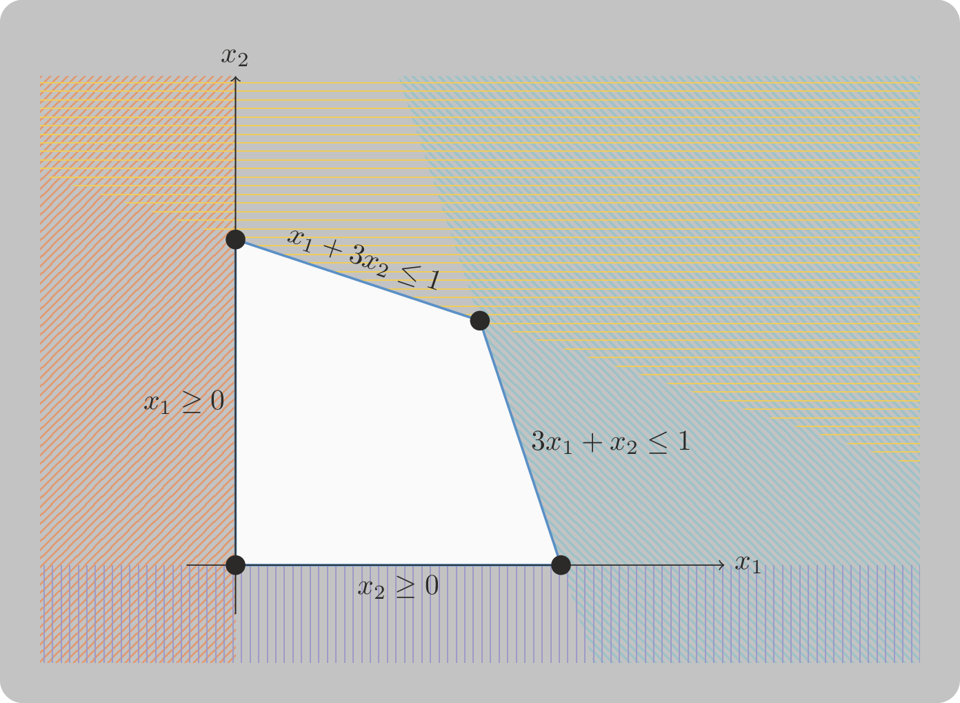
Figure A5.2:The same polytope shown in Figure A5.1, represented as the intersection of linear inequalities.
This second definition corresponds to:
The inequalities in (A5.3) define supporting half-spaces that together enclose the polytope.
Polytopes appear throughout mathematics, particularly in optimisation, where they form the feasible regions of linear programs. These connections are central to game theory, especially in the study of zero-sum games and general games.
While this example lives in , the techniques extend to higher-dimensional polytopes. The goal of this chapter is to develop tools for moving from vertex to vertex in such polytopes, an essential idea in both mathematical optimisation and algorithmic game theory.
Theory
Definition: Polytope as a Convex Hull
Let be a finite set of points. A polytope is the set of all convex combinations of points in :
Definition: Polytope as an Intersection of Half-Spaces
Let and . A polytope can also be defined as the set of points satisfying a system of linear inequalities:
The representation of a polytope as the intersection of half-spaces via will allow us to work efficiently with large systems.
Definition: Slack Variable
Given a system of linear inequalities of the form , a slack variable transforms each inequality into an equality by accounting for the difference between the left- and right-hand sides.
Formally, for each row , the inequality
can be rewritten as
where is the slack variable corresponding to the -th inequality.
Definition: Tableau Representation of Vertices
For and , given a system of linear inequalities:
This system of linear inequalities can be written as a system of equalities by adding slack variables to give a modified linear system of equalities:
Where and includes coefficients for the added slack variables:
Given the system a tableau is an extended matrix of the form:
This augmented matrix of the underlying linear system is used to represent points in Polytopes. Through elementary row operations which will be called pivots we can move from one vertex to another.
Example: Tableaux for the Motivating Example
The linear system for the Motivating Example is:
This corresponds to:
We can write a Tableau that represents the equivalent system of equations :
Tableaux are augmented matrices for linear systems, it is possible to do elementary row operations on them that do not modify the underlying system. We can also derive alternative tableaux from this example:
Multiplying 's row 1 by 3 and subtracting row 2 gives:
Multiplying 's row 2 by 8 and subtracting row 1 gives:
Multiplying 's row 1 by 9 and adding row 2 gives:
There are other tableaux that correspond to the same systems of equations but we next explore how tableaux correspond to vertices of polytopes. To do this we need a new definition:
Definition: Basic variables
A basic variable of a tableau corresponds to a column that is linearly independent from the others.
Example: Basic variables for the different Tableaux of the Motivating Example
The basic variables for:
The tableau (A5.14) are the two slack variables and .
The tableau (A5.15) are and .
The tableau (A5.16) are and .
The tableau (A5.17) are and .
Thus, the non-basic variables for:
The tableau (A5.14) are and .
The tableau (A5.15) are and .
The tableau (A5.16) are and .
The tableau (A5.17) are and .
Equivalence between a tableau and a vertex
A tableau represents the constraints and feasible region of a polytope. A given tableau represents a vertex of the polytope.
To obtain a vertex from the tableau:
Set the non basic variables to be 0;
Solve the remaining system of equations.
Example: equivalence between tableaux and vertices
For (A5.14): we set the non-basic variables to 0:
The remaining linear system from the tableau is:
Note that we do not need to solve this remaining linear system as setting the non-basic variables to 0 immediately gives us the vertex: (the origin of Figure A5.1).
For (A5.15): we set the non-basic variables to 0:
The remaining linear system from the tableau is:
Solving this gives: (the bottom right vertex of Figure A5.1).
For (A5.16): we set the non-basic variables to 0:
The remaining linear system from the tableau is:
Solving this gives: (the top right vertex of Figure A5.1).
For (A5.17): we set the non-basic variables to 0:
The remaining linear system from the tableau is:
Solving this gives: (the top left vertex of Figure A5.1).
We have recovered all four vertices from the 4 tableaux of Example: Tableaux for the Motivating Example. Note that in that example through the process of applying elementary row operations to the tableaux we moved across the edges of the polytope as shown in Figure A5.3.
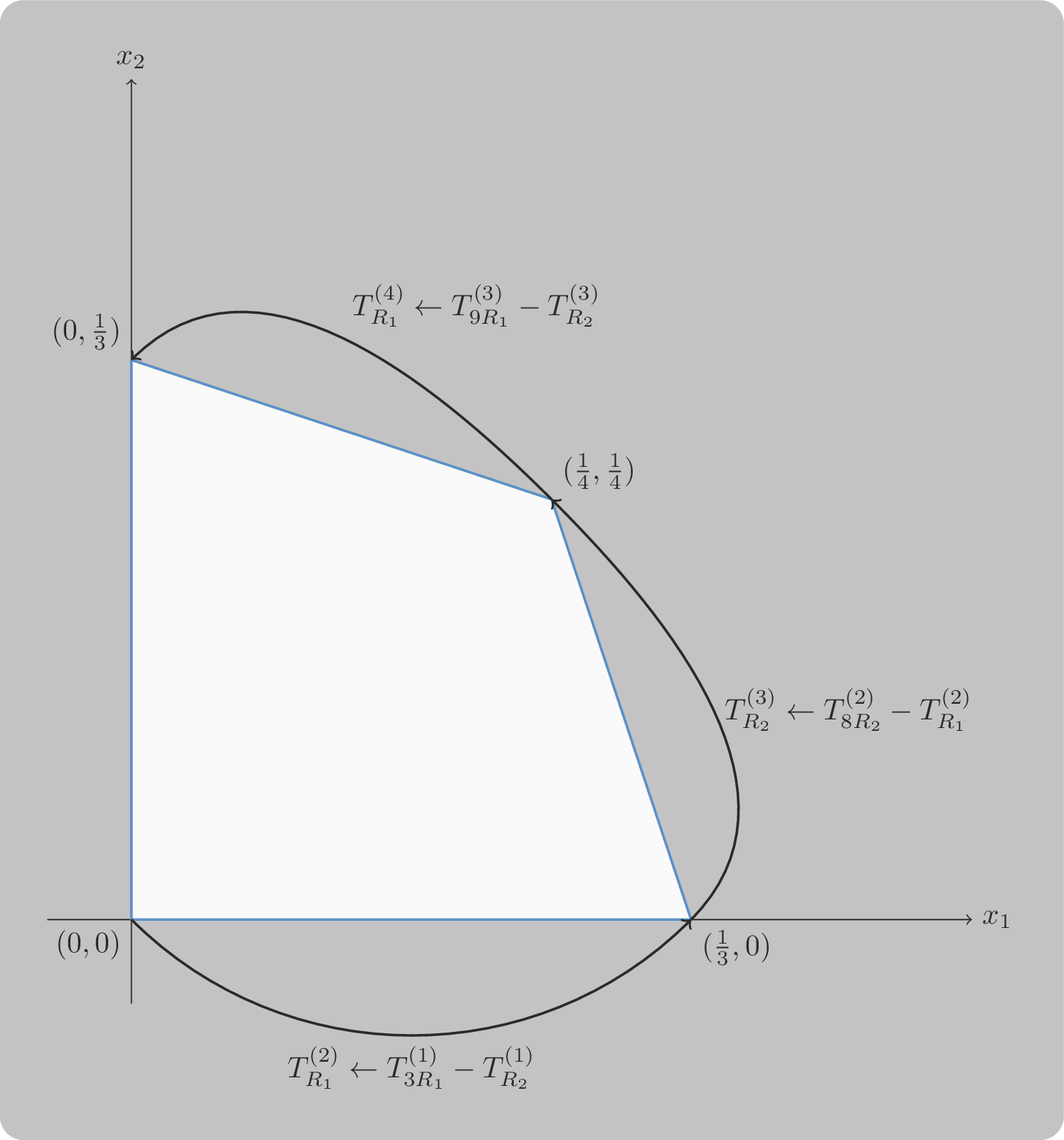
Figure A5.3:The two-dimensional polytope defined by (A5.1), with arrows showing the process of moving along the edges. The various row operations are written as short hand.
This process corresponds to making a non-basic variable basic and carefully choosing which basic variable to make non-basic.
Definition: Integer Pivoting
Pivoting is the process of updating a tableau by selecting one basic variable to leave the basis and one non-basic variable to enter it. This corresponds to performing row operations to rewrite the system so that the new basic variable appears with coefficient 1 in its row and 0 in all others.
In integer pivoting, we perform this process using only integer-preserving row operations, such as adding or subtracting integer multiples of rows. This is useful for maintaining exact arithmetic and geometric intuition in discrete settings.
Suppose you are given a tableau representing a system of equations and you choose a non-basic variable to enter the basis.
The goal is to perform a pivot so that becomes basic and one of the current basic variables is removed from the basis.
The pivot is carried out using the following steps:
Identify the pivot column Select the column of the tableau corresponding to .
Select the pivot row minimum ratio test For each row where the coefficient , compute the ratio:
(where corresponds to the final column of .)
Choose the row with the smallest non-negative ratio. The basic variable in this row will leave the basis.
Eliminate the pivot column in all other rows For each row , if necessary multiply it by a suitable integer multiplier and then subtract suitable integer multiples of row so that the entry in column becomes zero.
After these steps, the tableau reflects a new basic solution where is basic, and one previous basic variable has become non-basic.
Example: Moving from to 
Let us start at:
The non-basic variables are and . Let us choose to let become basic. This corresponds to the second column of the tableau.
Next we use the minimum ratio test:
The ratio for the first row:
The ratio for the second row:
Both of these are non-negative and the minimum value is obtained in the first row. Thus we pivot on the first row making the value in the second column and “all other rows” (in this case just the second row) 0.
Multiplying 's row 2 by 3 and subtracting row 1 gives:
Using Equivalence between a tableau and a vertex we set the basic variables to 0:
The remaining linear system from the tableau is:
Solving this gives: .
Exercises
Exercise: Polytope Representation
For each of the following sets of vertices:
Draw the corresponding polytope.
Write the polytope as the intersection of a set of halfspaces (i.e. inequalities).
Exercise: Basic and Non-Basic Variables
For each of the following tableaux, identify the basic and non-basic variables:
Exercise: Integer Pivoting
For the tableaux in Exercise: Basic and Non-Basic Variables:
For each non-basic variable, perform one step of integer pivoting:
Identify the pivot column;
Perform the minimum ratio test to determine the pivot row;
Execute the required row operations to complete the pivot.
Programming
Using SciPy to obtain the convex hull
The SciPy library has functionality to obtain the convex hull of a set of vertices.
import scipy.spatial
import numpy as np

V = [np.array([0, 0]), np.array([1 / 3, 0]), np.array([1 / 4, 1 / 4]),
np.array([0, 1 / 3])]
P = scipy.spatial.ConvexHull(V)
scipy.spatial.convex_hull_plot_2d(P);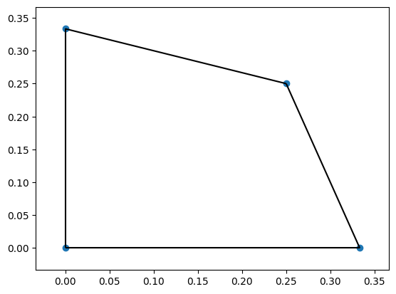
The obtained convex hull can be used to get the system of linear inequalities:
P.equationsarray([[-0. , -1. , 0. ],
[-1. , 0. , -0. ],
[ 0.9486833 , 0.31622777, -0.31622777],
[ 0.31622777, 0.9486833 , -0.31622777]])Using SciPy to obtain the half space
The Scipy library has functionality to obtain the vertices from a given intersection of half spaces.
First we create the system of linear inequalities , this is done passing: as single matrix
halfspace = np.array(
    (
        (-1, 0, 0),
        (0, -1, 0),
        (3, 1, -1),
        (1, 3, -1),
    )
)
We need to pass a point known to be in the interior of the Polytope. Now we can obtain the vertices the original vertices from (A5.1).
P = scipy.spatial.HalfspaceIntersection(halfspace, interior_point=np.array((1/5,
1/5)))
P.intersections
array([[2.77555756e-17, 3.33333333e-01],
[2.50000000e-01, 2.50000000e-01],
[0.00000000e+00, 0.00000000e+00],
[3.33333333e-01, 2.77555756e-17]])Carrying out row operations using NumPy
NumPy’s array operations allow for straightforward row operations.
T_1 = np.array(
    (
        (1, 3, 1, 0, 1),
        (3, 1, 0, 1, 1),
    )
)
T_2 = T_1
T_2[0] = 3 * T_2[0] - T_2[1]
T_2
array([[ 0, 8, 3, -1, 2],
[ 3, 1, 0, 1, 1]])Pivoting tableaux with Nashpy
NashPy has some internal functionality for integer pivoting, which at present is not designed to be user facing but is nonetheless useable:
import nashpy as nash

T = nash.linalg.Tableau(T_2)
Having created this tableau we can get the indices of the basic and non-basic variables:
T.basic_variables{0, 2}T.non_basic_variables{np.int64(1), np.int64(3)}We can pivot the tableau on a given column and given row:
T._pivot(column_index=1, pivot_row_index=1)This pivoted on the second column (index 1) returning which non-basic variable becomes basic as a result.
We can look at the tableau:
T._tableauarray([[-24, 0, 3, -9, -6],
[ 3, 1, 0, 1, 1]])Notable Research
The concept of pivoting and tableaux was first introduced by the mathematician George Dantzig in a 1947 report during his tenure at the Pentagon Dantzig, 1947.
The initial publication of this idea is found in Dantzig, 1951. Although Dantzig did not explicitly mention tableaux, they naturally emerged as an efficient method for traversing the edges of a polytope.
In Dantzig, 2020 (originally published in 1990), Dantzig shares the following anecdote:
"The first idea that would occur to anyone as a technique for solving a linear program, aside from the obvious one of moving through the interior of the convex set, is that of moving from one vertex to the next along the edges of the polyhedral set. I discarded this idea immediately as impractical in higher dimensional spaces. It seemed intuitively obvious that there would be far too many vertices and edges to wander over in the general case for such a method to be efficient.
When Hurwicz came to visit me at the Pentagon in the summer of 1947, I told him how I had discarded this vertex-edge approach as intuitively inefficient for solving LP. I suggested instead that we study the problem in the geometry of columns rather than the usual one of the rows -- column geometry incidentally was the one I had used in my Ph.D. thesis on the Neyman-Pearson Lemma. We dubbed the new method ‘climbing the bean pole.’"
A comprehensive historical overview is provided in Todd, 2002, which includes several other notable publications.
Two significant works connect integer pivoting to game theory:
In a 1951 book chapter, Dantzig established a connection for zero-sum games, as described in Adler, 2013.
Lemke & Howson, 1964 introduces the Lemke-Howson algorithm, which employs integer pivoting to find Nash equilibria in general games.
Conclusion
Integer pivoting offers a powerful lens through which to understand movement across the vertices of polytopes, providing a concrete foundation for key algorithms in linear programming and game theory. Through the tableau representation, we are able to:
Translate systems of inequalities into algebraic form;
Perform exact row operations that correspond to movement along polytope edges;
Interpret basic and non-basic variables as defining vertices and directions of movement.
These tools underpin the algorithms used for zero-sum games and Nash equilibrium computation.
Table A5.1 summarises the key concepts introduced in this appendix.
Table A5.1:Summary of integer pivoting
| Concept | Description |
|---|---|
| Polytope (convex hull) | Set of convex combinations of finite points |
| Polytope (half-spaces) | Set of solutions to a system of linear inequalities |
| Slack variable | Converts an inequality into an equality with a non-negative remainder |
| Tableau | Augmented matrix form of a linear system with slack variables |
| Basic variable | Variable corresponding to a pivot column; used to determine a vertex |
| Non-basic variable | Set to 0 when solving for vertex from tableau |
| Pivoting | Row operations used to exchange basic and non-basic variables |
| Minimum ratio test | Selects the pivot row to preserve feasibility during a pivot |
| Integer pivoting | Pivoting using only integer row operations to maintain exact structure |
Solutions
Solution to Exercise: Polytope Representation
1.
This is the unit square. As the intersection of half-spaces:
In standard form :
2.
We must find the convex hull of these four points. Computing the supporting half-spaces (using the convex hull):
The edges of the convex hull connect:
to : left edge, .
to : bottom edge. The line through these points has slope , giving , i.e., .
to : upper-left edge. Slope = . Line: , i.e., , giving .
to : upper-right edge. Slope = . Line: , i.e., .
to : see bottom edge above (they share the same bounding line together with ).
A complete half-space representation is:
import scipy.spatial
import numpy as np
import matplotlib.pyplot as plt

V1 = np.array([[0,0],[0,1],[1,0],[1,1]], dtype=float)
hull1 = scipy.spatial.ConvexHull(V1)
fig, axes = plt.subplots(1, 3, figsize=(9, 3))

for ax, V, title in zip(
    axes,
    [
        np.array([[0,0],[0,1],[1,0],[1,1]], dtype=float),
        np.array([[0,0],[0,1/4],[1,2/3],[2,1/5]], dtype=float),
        np.array([[0,0],[0,1/4],[1,2/3],[2,1/5],[1,0]], dtype=float),
    ],
    ["V1: unit square", "V2: 4 points", "V3: 5 points"]
):
    hull = scipy.spatial.ConvexHull(V)
    scipy.spatial.convex_hull_plot_2d(hull, ax=ax)
    ax.scatter(V[:, 0], V[:, 1], color="red", zorder=5)
    ax.set_title(title)

plt.tight_layout()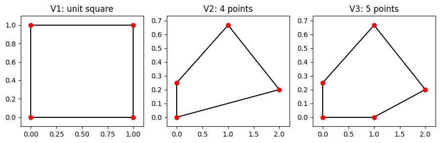
# Show the half-space inequalities for V2
V2 = np.array([[0,0],[0,1/4],[1,2/3],[2,1/5]], dtype=float)
hull2 = scipy.spatial.ConvexHull(V2)
print("Half-space equations for V2 (each row: [a, b, c] means a*x1 + b*x2 + c <= 0):")
print(hull2.equations)
Half-space equations for V2 (each row: [a, b, c] means a*x1 + b*x2 + c <= 0):
[[ 0.09950372 -0.99503719 -0. ]
[ 0.42288547 0.90618314 -1.02700756]
[-1. 0. -0. ]
[-0.38461538 0.92307692 -0.23076923]]
3.
The point lies inside or on the boundary of the convex hull of from part 2 (it is below the bottom edge at : , so is actually outside that edge). Adding changes the convex hull.
V3 = np.array([[0,0],[0,1/4],[1,2/3],[2,1/5],[1,0]], dtype=float)
hull3 = scipy.spatial.ConvexHull(V3)
print("Half-space equations for V3:")
print(hull3.equations)
print("\nVertices of hull3:", V3[hull3.vertices])
Half-space equations for V3:
[[ 0.42288547 0.90618314 -1.02700756]
[-1. 0. -0. ]
[-0.38461538 0.92307692 -0.23076923]
[-0. -1. 0. ]
[ 0.19611614 -0.98058068 -0.19611614]]
Vertices of hull3: [[2. 0.2 ]
[1. 0.66666667]
[0. 0.25 ]
[0. 0. ]
[1. 0. ]]
Solution to Exercise: Basic and Non-Basic Variables
1. For
The columns (from left to right) correspond to variables (or if these are slack variables). A basic variable corresponds to a column that has exactly one nonzero entry (a unit vector). Inspecting the columns:
Column 1 (): , a unit vector. Basic.
Column 2 (): , a unit vector. Basic.
Column 3 (): , not a unit vector. Non-basic.
Column 4 (): , not a unit vector. Non-basic.
Basic variables: . Non-basic variables: .
Setting non-basic variables to zero: , the system gives and , so the corresponding vertex is (if are the original variables, otherwise the vertex is in the coordinates).
2. For
Column 1 (): , not a unit vector. Non-basic.
Column 2 (): , not a unit vector. Non-basic.
Column 3 (): , a unit vector. Basic.
Column 4 (): , a unit vector. Basic.
Basic variables: . Non-basic variables: .
Setting non-basic variables to zero: , and from the last column, , . This corresponds to the origin vertex.
Solution to Exercise: Integer Pivoting
We perform integer pivoting on each non-basic variable for the two tableaux from the exercise above.
Pivoting on : The non-basic variables are and .
Pivot on (column 3):
The pivot column entries are . Both are positive, so we apply the minimum ratio test:
Row 1:
Row 2:
The minimum ratio is in row 1, so we pivot on row 1.
To eliminate from row 2 by integer pivoting (as defined in Definition: Integer Pivoting), multiply row 2 by 5 and subtract 4 times row 1, zeroing out column 3 in row 2:
The updated tableau is:
The basic variables are now (from row 1) and (from row 2). Setting non-basic variables : from row 1, ; from row 2, .
Pivot on (column 4) of :
The pivot column entries are . Both positive. Minimum ratio test:
Row 1:
Row 2:
Minimum is in row 2. Pivot on row 2. Eliminate from row 1: multiply row 1 by 9 and subtract row 2 (integer pivoting):
The updated tableau is:
Pivoting on : The non-basic variables are and .
Pivot on (column 1):
The pivot column entries are . Both positive. Minimum ratio test:
Row 1:
Row 2:
Minimum is in row 2. Pivot on row 2. Eliminate from row 1:
The updated tableau is:
Basic variables are now (row 2) and (row 1). Setting : from row 2, .
Pivot on (column 2):
Starting from , the pivot column entries are . Both positive. Minimum ratio test:
Row 1:
Row 2:
Minimum is in row 1. Pivot on row 1. Eliminate from row 2:
The updated tableau is:
Basic variables are now (row 1) and (row 2). Setting : from row 1, ; from row 2, ... Actually with : row 1 gives .
import numpy as np

# Tableau T^(a)
T_a = np.array([[1, 0, 5, 1, 1],
                [0, 1, 4, 9, 1]], dtype=float)

# Pivot on column 3 (index 2), pivot row 1 (index 0): minimum ratio 1/5
T_a_pivot_x3 = T_a.copy()
pivot_col, pivot_row = 2, 0
# new_row2 = 5*row2 - 4*row1 (to zero column 3 in row 2)
T_a_pivot_x3[1] = T_a[1] * T_a[0, pivot_col] - T_a[0] * T_a[1, pivot_col]
print("T^(a) after pivot on x3 (col 3, row 1):")
print(T_a_pivot_x3)

# Pivot on column 4 (index 3) of T^(a), pivot row 2 (index 1): minimum ratio 1/9
T_a_pivot_x4 = T_a.copy()
pivot_col, pivot_row = 3, 1
# new_row1 = 9*row1 - row2 (to zero column 4 in row 1)
T_a_pivot_x4[0] = T_a[0] * T_a[1, pivot_col] - T_a[1] * T_a[0, pivot_col]
print("\nT^(a) after pivot on x4 (col 4, row 2):")
print(T_a_pivot_x4)
T^(a) after pivot on x3 (col 3, row 1):
[[ 1. 0. 5. 1. 1.]
[-4. 5. 0. 41. 1.]]
T^(a) after pivot on x4 (col 4, row 2):
[[ 9. -1. 41. 0. 8.]
[ 0. 1. 4. 9. 1.]]
# Tableau T^(b)
T_b = np.array([[4, 8, 1, 0, 1],
                [8, 1, 0, 1, 1]], dtype=float)

# Pivot on x1 (col 1, index 0), pivot row 2 (index 1): minimum ratio 1/8
T_b_pivot_x1 = T_b.copy()
pivot_col, pivot_row = 0, 1
T_b_pivot_x1[0] = T_b[0] * T_b[1, pivot_col] - T_b[1] * T_b[0, pivot_col]
print("T^(b) after pivot on x1 (col 1, row 2):")
print(T_b_pivot_x1)

# Pivot on x2 (col 2, index 1), pivot row 1 (index 0): minimum ratio 1/8
T_b_pivot_x2 = T_b.copy()
pivot_col, pivot_row = 1, 0
T_b_pivot_x2[1] = T_b[1] * T_b[0, pivot_col] - T_b[0] * T_b[1, pivot_col]
print("\nT^(b) after pivot on x2 (col 2, row 1):")
print(T_b_pivot_x2)
T^(b) after pivot on x1 (col 1, row 2):
[[ 0. 60. 8. -4. 4.]
[ 8. 1. 0. 1. 1.]]
T^(b) after pivot on x2 (col 2, row 1):
[[ 4. 8. 1. 0. 1.]
[60. 0. -1. 8. 7.]]
- Dantzig, G. B. (1947). Maximization of a Linear Function of Variables Subject to Linear Inequalities (Techreport P-38). Rand Corporation.
- Dantzig, G. B. (1951). Maximization of a linear function of variables subject to linear inequalities. Activity Analysis of Production and Allocation, 13, 339–347.
- Dantzig, G. B. (2020). Impact of linear programming on computer development. In Computers in Mathematics (pp. 233–240). CRC Press.
- Todd, M. J. (2002). The many facets of linear programming. Mathematical Programming, 91(3), 417–436.
- Adler, I. (2013). The equivalence of linear programs and zero-sum games. International Journal of Game Theory, 42, 165–177.
- Lemke, C. E., & Howson, J. T., Jr. (1964). Equilibrium points of bimatrix games. Journal of the Society for Industrial and Applied Mathematics, 12(2), 413–423.