Nash Equilibrium - Game Theory

When every player’s strategy is a best response to every other’s, no one has an incentive to deviate unilaterally. This configuration is called a Nash equilibrium. This chapter formalises the concept, establishes its existence, and develops a systematic algorithm for computing it.

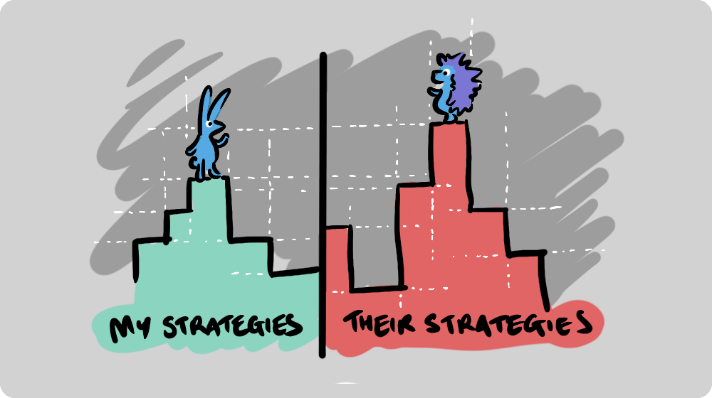
Two creatures, each sitting at the peak of their own best response landscape. — Figure 1:Each player climbs their own landscape of strategies, one shaped by what the other player does. At a Nash equilibrium both have reached the top of their respective hill: each is already standing on its best response to where the other stands, so neither has anywhere better to go.

Motivating Example¶

In the coordination Game (3), in how many situations do neither player have an incentive to independently change their strategy?

Neither player having a reason to change their strategy implies that both strategies are best responses to each other.

Recall that for the Coordination game is defined by:

M_r = \begin{pmatrix} 3 & 1 \\ 0 & 2 \end{pmatrix} \qquad M_c = \begin{pmatrix} 2 & 1 \\ 0 & 3 \end{pmatrix}

(1)

If we consider strategies that only play a single action, there are two options for each strategy:

\sigma_1 \in \{(1, 0), (0, 1)\}

(2)

and:

\sigma_2 \in \{(1, 0), (0, 1)\}

(3)

We will inspect all four combinations:

$\sigma_1 = (1, 0)$ and $\sigma_2 = (1, 0)$ corresponds to both players playing their first action, which gives: $u_r(\sigma_1, \sigma_2) = 3$ and $u_c(\sigma_1, \sigma_2) = 2$ .
If the row player were to modify their strategy (while the column player stayed unchanged) to play the second action, their utility would decrease. Likewise, if the column player were to modify their strategy, their utility would also decrease.
$\sigma_1 = (1, 0)$ and $\sigma_2 = (0, 1)$ corresponds to the row player playing their first action and the column player playing their second action, which gives: $u_r(\sigma_1, \sigma_2) = 1$ and $u_c(\sigma_1, \sigma_2) = 1$ .
In this case, if either player were to move, their utility would increase.
$\sigma_1 = (0, 1)$ and $\sigma_2 = (1, 0)$ corresponds to the row player playing their second action and the column player playing their first action, which gives: $u_r(\sigma_1, \sigma_2) = 0$ and $u_c(\sigma_1, \sigma_2) = 0$ .
In this case, if either player were to move, their utility would increase.
$\sigma_1 = (0, 1)$ and $\sigma_2 = (0, 1)$ corresponds to both players playing their second action, which gives: $u_r(\sigma_1, \sigma_2) = 2$ and $u_c(\sigma_1, \sigma_2) = 3$ .
If the row player were to modify their strategy (while the column player stayed unchanged), their utility would decrease. Likewise, if the column player were to modify their strategy, their utility would also decrease.

Is there another pair of strategies that are best responses to each other and will such a pair always exist for any game?

Theory¶

A pair of strategies that are best responses to each other is a Nash equilibrium.

Definition: Nash Equilibria¶

In an $N$ -player normal form game, a Nash equilibrium is a strategy profile
$\tilde{s} = (\tilde{s}_1, \tilde{s}_2, \dots, \tilde{s}_N)$ such that:

u_i(\tilde{s}) = \max_{\bar{s}_i \in \Delta(\mathcal{A}_i)} u_i(\bar{s}_i, \tilde{s}_{-i}) \quad \text{for all } i

(4)

Theorem: Existence of Nash Equilibrium¶

Every finite $N$ -player normal form game has at least one Nash equilibrium.

Proof sketch¶

The proof, due to Nash Jr, 1950, applies Kakutani’s fixed-point theorem Kakutani, 1941 to the best response correspondence. For each player $i$ , define:

\beta_i(s_{-i}) = \arg\max_{\sigma_i \in \Delta(\mathcal{A}_i)} u_i(\sigma_i, s_{-i})

(5)

Here $\beta_i(s_{-i})$ is the set of all mixed strategies for player $i$ that are best responses to the opponents’ strategies $s_{-i}$ . The joint best response correspondence $\beta: \prod_i \Delta(\mathcal{A}_i) \to \prod_i \Delta(\mathcal{A}_i)$ satisfies the conditions of Kakutani’s theorem (strategy spaces are compact and convex, and $\beta$ has a closed graph and convex values), so a fixed point $\tilde{s}$ exists. Any fixed point satisfies $\tilde{s}_i \in \beta_i(\tilde{s}_{-i})$ for all $i$ , which is precisely the Nash equilibrium condition.

The following algorithm gives an approach to use the best response condition to systematically find all Nash equilibrium.

Definition: Support Enumeration Algorithm¶

The algorithm proceeds as follows:

For a two-player game $(M_r, M_c) \in \left(\mathbb{R}^{m \times n}\right)^2$ , the following algorithm returns all pairs of best responses:

For all pairs of supports (subsets of the action space) $(I, J)$ :
Solve the following equations (to ensure best responses):
- $\sum_{i \in I} {\sigma_{r}}_i {M_{c}}\_{ij} = v \quad \text{for all } j \in J$
- $\sum_{j \in J} {M_r}_{ij} {\sigma\_{c}}\_j = u \quad \text{for all } i \in I$
Solve the normalisation and non-negativity constraints:
- $\sum_{i=1}^m {\sigma_{r}}_i = 1$ and ${\sigma_1}_i \geq 0$ for all $i$
- $\sum_{j=1}^n {\sigma_{c}}_j = 1$ and ${\sigma_2}_j \geq 0$ for all $j$
Check the best response condition.

Repeat steps 2–4 for all potential pairs of actions.

Example: Support enumeration algorithm for the coordination game¶

Let us apply the support enumeration algorithm to the coordination game.

The following supports (subsets of the action space) need to be considered:

I \in \{\{r_1\}, \{r_2\}, \{r_1, r_2\}\}

(6)

and

J \in \{\{c_1\}, \{c_2\}, \{c_1, c_2\}\}

(7)

For the cases where $|I|=|J|=1$ steps 2, 3 and 4 of the support enumeration algorithm correspond to finding best responses in the action space. This can be done by highlighting best responses:

M_r = \begin{pmatrix} \underline{3} & 1 \\ 0 & \underline{2} \end{pmatrix} \qquad M_c = \begin{pmatrix} \underline{2} & 1 \\ 0 & \underline{3} \end{pmatrix}

(8)

The support enumeration algorithm for $|I|=|J|=1$ gives the two following Nash equilibria:

((1, 0), (1, 0)) \qquad ((0, 1), (0, 1))

(9)

The final pair of actions to consider is when $I=(r_1, r_2)$ and $J=(c_1, c_2)$ . In this case let:

\sigma_1=(x, 1 - x)\qquad \sigma_2=(y,1-y)

(10)

for $0 < x < 1$ and $0 < y < 1$ .

Step 2 corresponds to setting:

\begin{align*} \sum_{i \in I} {\sigma_{r}}_i {M_{c}}_{i1} = 2 x + 0 (1-x) &= v\\ \sum_{i \in I} {\sigma_{r}}_i {M_{c}}_{i2} = 1 x + 3 (1 -x) &= v \end{align*}

(11)

and

\begin{align*} \sum_{j \in J} {M_r}_{1j} {\sigma_{c}}_j = 3y + 1(1-y) &= u \\ \sum_{j \in J} {M_r}_{2j} {\sigma_{c}}_j = 0y + 2(1-y) &= u \\ \end{align*}

(12)

The particular values of $u$ or $v$ are not required so we can equate these pairs of expressions:

\begin{align*} 2x = x + 3-3x &\implies x =\frac{3}{4}\\ 3y + 1-y = 2 - 2y &\implies y =\frac{1}{4}\\ \end{align*}

(13)

Giving: $\sigma_1 = (3/4, 1/4)$ and $\sigma_2=(1/4, 3/4)$ .

Step 3 already holds as we enforced $\sigma_1 = (x, 1 - x)$ and $\sigma_2 = (y, 1 - y)$ at the start of our calculations. This is not necessarily the case for larger games.

The final step, step 4, requires us to check the best response condition. This is to check that there exists no better choice of action outside of the chosen set of $I$ and $J$ . This is more relevant for games with larger action spaces but let us nonetheless carry out the calculations:

M_r \sigma_2^\mathsf{T}= \begin{pmatrix}3/2 \\ 3/2\end{pmatrix}

(14)

and

\sigma_1 M_c = \begin{pmatrix}3/2 & 3/2\end{pmatrix}

(15)

as required by the best response condition. The support enumeration algorithm has given 3 Nash equilibria:

\left\{ ((1, 0), (1, 0)), ((0, 1), (0, 1)), ((\frac{3}{4}, \frac{1}{4}), (\frac{1}{4}, \frac{3}{4})), \right\}

(16)

The support enumeration algorithm is one of many algorithms that can be used to compute Nash equilibrium. Like most of the algorithms it works well for “most” games. When games are “degenerate” it may need more calculations and fail to give all equilibria.

Definition: Degenerate Games¶

A two player game is called non degenerate if no strategy of support size $k$ has more than $k$ best response actions.

Example: Support Enumeration for a degenerate game¶

Let us use support enumeration for the following game.

M_r = \begin{pmatrix} 2 & 5 \\ 0 & 5\\ \end{pmatrix} \qquad M_c = \begin{pmatrix} 2 & 1 \\ 0 & 1\\ \end{pmatrix}

(17)

First, we note that this game is degenerate, there are two best responses in action space to the first column:

M_r = \begin{pmatrix} \underline{2} & \underline{5} \\ 0 & \underline{5}\\ \end{pmatrix} \qquad M_c = \begin{pmatrix} \underline{2} & 1 \\ 0 & \underline{1}\\ \end{pmatrix}

(18)

Evaluating best responses in action space gives Nash equilibria:

((1, 0), (1, 0)) \qquad ((0, 1), (0, 1))

(19)

We need to consider new pairs of supports:

$\sigma_1=(x, 1-x)$ and $\sigma_2 = (1, 0)$ : there is single best response to the first column so nothing else to consider here.
$\sigma_1=(x, 1-x)$ and $\sigma_2 = (0, 1)$ : step 2 holds for all $x$ , step 3 is already satisfied (the vectors are both probability distributions) thus we are left to check the best response condition:
$\sigma_1M_c=(2x, 1)$
(20)
the only value of $x$ that gives a pair of best response is when the column player has no incentive to move from the support thus $2x=1 \implies x=1/2$ .

Exercises¶

Exercise 2

A soccer player (Player 1) is taking a penalty kick and can shoot either left or right: $S_1 = \{\text{SL}, \text{SR}\}$ . The goalie (Player 2) can dive left or right: $S_2 = \{\text{DL}, \text{DR}\}$ . The probabilities of scoring a goal (depending on the chosen strategies) are shown in the matrix below:

\begin{pmatrix} 0.8 & 0.15 \\ 0.2 & 0.95 \end{pmatrix}

(23)

Assume the utility to Player 1 is the probability of scoring, and the utility to Player 2 is the probability of preventing a goal. What is the Nash equilibrium of this game?

Now suppose Player 1 has a third strategy: shooting in the middle. The new action set becomes $S_1 = \{\text{SL}, \text{SM}, \text{SR}\}$ . The updated probability matrix is:

\begin{pmatrix} 0.8 & 0.15 \\ 0.5 & 0.5 \\ 0.2 & 0.95 \end{pmatrix}

(24)

Determine the new Nash equilibrium for the extended game.

Programming¶

The Nashpy library has an implementation of the support enumeration algorithm. First let us create the payoff matrices and the game:

import numpy as np
import nashpy as nash

A = np.array(
    (
        (3, 1),
        (0, 2),
    )
)
B = np.array(
    (
        (2, 1),
        (0, 3),
    )
)

coordination_game = nash.Game(A, B)
print(coordination_game)

Bi matrix game with payoff matrices:

Row player:
[[3 1]
 [0 2]]

Column player:
[[2 1]
 [0 3]]

Now to use the support enumeration algorithm:

print(list(coordination_game.support_enumeration()))

[(array([1., 0.]), array([1., 0.])), (array([0., 1.]), array([0., 1.])), (array([0.75, 0.25]), array([0.25, 0.75]))]

Notable Research¶

Support enumeration is as close to a “from first principles” algorithm for computing Nash equilibria. Thus there is no specific paper to point to as per its formulation. Or indeed there is no specific set of papers that use it for their findings although a lot of papers that consider small games are in essence using support enumeration.

For example in Chiappori et al., 2002 theoretical results are given regarding penalty kicks that rely on the indifference ensured by the best response condition which is in turn essentially an application of the support enumeration algorithm.

A similar paper applied to another animal conservation is Lee & Roberts, 2016 in which the authors build a theoretical model of the effectiveness of Rhino horn devaluation. Once again the calculation presented are essentially an application of the support enumeration algorithm.

In Knight et al., 2017 whilst a different algorithm is used to identify Nash equilibrium for strategic hospital interactions it is somewhat similar to the support enumeration algorithm except that it takes advantage of the specific structure of the game considered.

Conclusion¶

This chapter introduced the concept of Nash equilibrium and demonstrated a
systematic method for identifying all equilibria in a two-player game using the
support enumeration algorithm. This method is rooted directly in the best
response condition and provides a computational approach that works well for
many games, particularly when the number of actions is small.

The support enumeration algorithm is conceptually simple but becomes expensive as action spaces grow; it is most useful for small games.

Table 1 summarises the core concepts introduced in this chapter.

Table 1:The main concepts of Nash equilibrium

Concept	Description
Nash equilibrium	A strategy profile where each player’s strategy is a best response to the others’
Support of a strategy	The set of actions played with positive probability
Support enumeration algorithm	Enumerates possible supports and checks conditions for equilibrium
Degenerate game	A game in which some strategy of support size $k$ has more than $k$ best responses

Solutions¶

Solution to Exercise 1 #

We apply the support enumeration algorithm to find all Nash equilibria.

Game 1:

A = \begin{pmatrix} 3 & 3 & 2 \\ 2 & 1 & 3 \end{pmatrix} \qquad B = \begin{pmatrix} 2 & 1 & 3 \\ 2 & 3 & 2 \end{pmatrix}

(25)

The row player has 2 actions ( $r_1, r_2$ ) and the column player has 3 actions ( $c_1, c_2, c_3$ ).

Pure strategy Nash equilibria.

Best responses for the row player: $r_1$ is a best response to $c_1$ ( $3 > 2$ ) and $c_2$ ( $3 > 1$ ); $r_2$ is a best response to $c_3$ ( $3 > 2$ ).

Best responses for the column player: $c_3$ is a best response to $r_1$ ( $3 > 2 > 1$ ); $c_2$ is a best response to $r_2$ ( $3 > 2 = 2$ ).

There are no mutual best response pairs, so no pure strategy Nash equilibrium exists.

Mixed strategy supports.

This game is non-degenerate, so no strategy of support size $k$ has more than $k$ best responses. With $|I| = 2$ , the column player can have at most 2 best responses, so supports with $|J| = 3$ need not be considered.

$I = \{r_1, r_2\}$ , $J = \{c_1, c_2\}$ : Let $\sigma_c = (y_1, y_2, 0)$ with $y_1 + y_2 = 1$ . Row player indifference requires $3y_1 + 3y_2 = 2y_1 + y_2$ , giving $3 = y_1 + 1$ , so $y_1 = 2$ . Invalid.

$I = \{r_1, r_2\}$ , $J = \{c_1, c_3\}$ : Let $\sigma_c = (y_1, 0, y_3)$ with $y_1 + y_3 = 1$ .

Row player indifference: $3y_1 + 2y_3 = 2y_1 + 3y_3 \implies y_1 = y_3 = \tfrac{1}{2}$ .

Column player indifference: $2x + 2(1-x) = 3x + 2(1-x) \implies 2 = x + 2 \implies x = 0$ . Contradicts support $\{r_1, r_2\}$ . No NE.

$I = \{r_1, r_2\}$ , $J = \{c_2, c_3\}$ : Let $\sigma_c = (0, y_2, y_3)$ with $y_2 + y_3 = 1$ .

Row player indifference: $3y_2 + 2y_3 = y_2 + 3y_3 \implies 2y_2 = y_3$ .

With $y_2 + y_3 = 1$ : $y_2 = \tfrac{1}{3}$ , $y_3 = \tfrac{2}{3}$ .

Column player indifference: $x + 3(1-x) = 3x + 2(1-x) \implies 3 - 2x = x + 2 \implies x = \tfrac{1}{3}$ .

Both $x$ and $(y_2, y_3)$ are valid probability distributions. Checking the best response condition:

A \sigma_c^T = \begin{pmatrix} 3 & 3 & 2 \\ 2 & 1 & 3 \end{pmatrix} \begin{pmatrix} 0 \\ 1/3 \\ 2/3 \end{pmatrix} = \begin{pmatrix} 7/3 \\ 7/3 \end{pmatrix}

(26)

\sigma_r B = \begin{pmatrix} 1/3 & 2/3 \end{pmatrix} \begin{pmatrix} 2 & 1 & 3 \\ 2 & 3 & 2 \end{pmatrix} = \begin{pmatrix} 2 & 7/3 & 7/3 \end{pmatrix}

(27)

Both rows give equal payoff $7/3$ , and column $c_1$ (outside the support) gives $2 < 7/3$ , so the best response condition is satisfied.

Nash equilibria for Game 1:

\left\{ \left(\left(\frac{1}{3}, \frac{2}{3}\right),\ \left(0, \frac{1}{3}, \frac{2}{3}\right)\right) \right\}

(28)

Here is some code to confirm the calculation:

import nashpy as nash
import numpy as np

A = np.array([[3, 3, 2], [2, 1, 3]])
B = np.array([[2, 1, 3], [2, 3, 2]])
game_1 = nash.Game(A, B)
for eq in game_1.support_enumeration():
    print(eq)

(array([0.33333333, 0.66666667]), array([0.        , 0.33333333, 0.66666667]))

Game 2:

A = \begin{pmatrix} 3 & -1 \\ 2 & 7 \end{pmatrix} \qquad B = \begin{pmatrix} -3 & 1 \\ 1 & -6 \end{pmatrix}

(29)

Pure strategy Nash equilibria.

Row player: $r_1$ is a best response to $c_1$ ( $3 > 2$ ); $r_2$ is a best response to $c_2$ ( $7 > -1$ ). Column player: $c_2$ is a best response to $r_1$ ( $1 > -3$ ); $c_1$ is a best response to $r_2$ ( $1 > -6$ ). There are no mutual best response pairs, so no pure NE exists.

Mixed strategy with $I = \{r_1, r_2\}$ , $J = \{c_1, c_2\}$ :

Let $\sigma_r = (x, 1-x)$ and $\sigma_c = (y, 1-y)$ .

Row player indifference:

3y - (1-y) = 2y + 7(1-y) \implies 4y - 1 = 7 - 5y \implies y = \frac{8}{9}

(30)

Column player indifference:

-3x + (1-x) = x - 6(1-x) \implies 1 - 4x = 7x - 6 \implies x = \frac{7}{11}

(31)

Both values lie in $(0,1)$ . Checking the best response condition:

A \sigma_c^T = \begin{pmatrix} 3 & -1 \\ 2 & 7 \end{pmatrix} \begin{pmatrix} 8/9 \\ 1/9 \end{pmatrix} = \begin{pmatrix} 23/9 \\ 23/9 \end{pmatrix}

(32)

\sigma_r B = \begin{pmatrix} 7/11 & 4/11 \end{pmatrix} \begin{pmatrix} -3 & 1 \\ 1 & -6 \end{pmatrix} = \begin{pmatrix} -17/11 & -17/11 \end{pmatrix}

(33)

Both rows and both columns yield equal payoffs, confirming the equilibrium.

Nash equilibria for Game 2:

\left\{ \left(\left(\frac{7}{11}, \frac{4}{11}\right),\ \left(\frac{8}{9}, \frac{1}{9}\right)\right) \right\}

(34)

Here is some code to confirm the calculations:

A = np.array([[3, -1], [2, 7]])
B = np.array([[-3, 1], [1, -6]])
game_2 = nash.Game(A, B)
for eq in game_2.support_enumeration():
    print(eq)

(array([0.63636364, 0.36363636]), array([0.88888889, 0.11111111]))

Solution to Exercise 2 #

The payoff matrices are:

M_r = \begin{pmatrix} 0.8 & 0.15 \\ 0.2 & 0.95 \end{pmatrix} \qquad M_c = \begin{pmatrix} 0.2 & 0.85 \\ 0.8 & 0.05 \end{pmatrix}

(35)

where $M_c = 1 - M_r$ since the goalkeeper’s utility is the probability of saving.

Pure strategy best responses.

Row player: SL is a best response to DL ( $0.8 > 0.2$ ); SR is a best response to DR ( $0.95 > 0.15$ ). Column player: DR is a best response to SL ( $0.85 > 0.20$ ); DL is a best response to SR ( $0.8 > 0.05$ ). There are no mutual best response pairs, so no pure NE exists.

Mixed strategy NE with $I = \{\text{SL}, \text{SR}\}$ , $J = \{\text{DL}, \text{DR}\}$ :

Let $\sigma_1 = (x, 1-x)$ and $\sigma_2 = (y, 1-y)$ .

Kicker indifference:

0.8y + 0.15(1-y) = 0.2y + 0.95(1-y) \implies 1.4y = 0.8 \implies y = \frac{4}{7}

(36)

Goalkeeper indifference:

0.2x + 0.8(1-x) = 0.85x + 0.05(1-x) \implies 0.75 = 1.4x \implies x = \frac{15}{28}

(37)

Both values lie in $(0,1)$ . The Nash equilibrium of the two-action game is:

\sigma_1^* = \left(\frac{15}{28},\ \frac{13}{28}\right) \qquad \sigma_2^* = \left(\frac{4}{7},\ \frac{3}{7}\right)

(38)

import nashpy as nash
import numpy as np

M_r = np.array([[0.8, 0.15], [0.2, 0.95]])
M_c = 1 - M_r
two_action_game = nash.Game(M_r, M_c)
for eq in two_action_game.support_enumeration():
    print(eq)

(array([0.53571429, 0.46428571]), array([0.57142857, 0.42857143]))

Extended game with $S_1 = \{\text{SL},\ \text{SM},\ \text{SR}\}$ :

M_r = \begin{pmatrix} 0.8 & 0.15 \\ 0.5 & 0.5 \\ 0.2 & 0.95 \end{pmatrix} \qquad M_c = \begin{pmatrix} 0.2 & 0.85 \\ 0.5 & 0.5 \\ 0.8 & 0.05 \end{pmatrix}

(39)

There is no pure NE by the same cycling argument as before. We check each possible kicker support against $J = \{\text{DL}, \text{DR}\}$ .

Support $\{\text{SL}, \text{SR}\}$ : The equilibrium $\sigma_2^* = (4/7, 3/7)$ from the two-action game remains a candidate. We verify SM is not a profitable deviation for the kicker:

u_r(\text{SM},\ \sigma_2^*) = 0.5 \cdot \tfrac{4}{7} + 0.5 \cdot \tfrac{3}{7} = 0.5

(40)

u_r(\text{SL},\ \sigma_2^*) = 0.8 \cdot \tfrac{4}{7} + 0.15 \cdot \tfrac{3}{7} = \tfrac{3.65}{7} \approx 0.521

(41)

Since $0.5 < 0.521$ , SM is not a best response, so $\sigma_1^* = (15/28,\ 0,\ 13/28)$ and $\sigma_2^* = (4/7,\ 3/7)$ is a valid NE.

Support $\{\text{SL}, \text{SM}\}$ : Goalkeeper indifference requires $0.2\, x_{\text{SL}} + 0.5\, x_{\text{SM}} = 0.85\, x_{\text{SL}} + 0.5\, x_{\text{SM}}$ , which gives $x_{\text{SL}} = 0$ . Contradicts the support. No NE.

Support $\{\text{SM}, \text{SR}\}$ : Goalkeeper indifference requires $x_{\text{SR}} = 0$ . Contradicts the support. No NE.

Support $\{\text{SL}, \text{SM}, \text{SR}\}$ : Kicker indifference requires SL $=$ SM $=$ SR under $\sigma_2 = (y, 1-y)$ . From SL $=$ SR we get $y = 4/7$ , but from SL $=$ SM we get $y = 7/13 \neq 4/7$ . No full-support NE exists.

Conclusion: The unique Nash equilibrium in the extended game is:

\sigma_1^* = \left(\frac{15}{28},\ 0,\ \frac{13}{28}\right), \qquad \sigma_2^* = \left(\frac{4}{7},\ \frac{3}{7}\right)

(42)

The middle shot is never played at equilibrium because its scoring probabilities are dominated by the mixing of SL and SR, giving the kicker no strategic advantage from including it. This can been seen numerically by plotting the utilities as a function of the $\sigma_2=(y, 1-y)$ . At no value of $y$ is the middle shot ever a best response.

import matplotlib.pyplot as plt

M_r = np.array([[0.8, 0.15], [0.5, 0.5], [0.2, 0.95]])

plt.plot(M_r[0], label=r"$u_r(\text{SL}, \sigma_2)$")
plt.plot(M_r[1], label=r"$u_r(\text{SM}, \sigma_2)$")
plt.plot(M_r[2], label=r"$u_r(\text{SR}, \sigma_2)$")
plt.xlabel("$y$")
plt.legend()

Let us confirm the equilibria:

M_c = 1 - M_r
three_action_game = nash.Game(M_r, M_c)
for eq in three_action_game.support_enumeration():
    print(eq)

(array([0.53571429, 0.        , 0.46428571]), array([0.57142857, 0.42857143]))

References¶

Nash Jr, J. F. (1950). Equilibrium points in n-person games. Proceedings of the National Academy of Sciences, 36(1), 48–49.
Kakutani, S. (1941). A generalization of Brouwer’s fixed point theorem. Duke Mathematical Journal, 8(3), 457–459.
Chiappori, P.-A., Levitt, S., & Groseclose, T. (2002). Testing mixed-strategy equilibria when players are heterogeneous: The case of penalty kicks in soccer. American Economic Review, 92(4), 1138–1151.
Lee, T. E., & Roberts, D. L. (2016). Devaluing rhino horns as a theoretical game. Ecological Modelling, 337, 73–78.
Knight, V., Komenda, I., & Griffiths, J. (2017). Measuring the price of anarchy in critical care unit interactions. Journal of the Operational Research Society, 68(6), 630–642.