Replicator Dynamics - Game Theory

When strategies that perform well spread and those that perform poorly shrink, populations evolve. This chapter derives the replicator dynamics equation, which models this selection process mathematically, and analyses the equilibria and long-run behaviour it produces.

Motivating Example: Coffee clubs and the common good game¶

Across a large university campus, students form informal coffee clubs. Each day, students join clubs to share a cafetière of coffee and discuss algebraic topology or the latest student gossip. There are three types of students:

Cooperators always bring a scoop of ground coffee to the club.
Defectors show up empty-handed but still drink the coffee.
Loners prefer to skip clubs and enjoy a quiet cup alone, reliable, if a bit less exciting.

In each club, all coffee brought is pooled, brewed, and the resulting pot is shared equally among the attendees. If there are $k$ cooperators, the pot yields $rk$ units of value to be divided among all participants (cooperators and defectors). The loners, who don’t attend clubs, receive a fixed payoff $\sigma$ .

Let the total population be normalized to 1, with:

$x_c$ the proportion of cooperators,
$x_d$ the proportion of defectors,
$x_z = 1 - x_c - x_d$ the proportion of loners.

Assuming the population is large and well-mixed, we can model the average payoff to each strategy as:

$f_c(x) = r \cdot \frac{x_c}{x_c + x_d} - 1$
$f_d(x) = r \cdot \frac{x_c}{x_c + x_d}$
$f_l(x) = \sigma$

Here, $r > 1$ is the return factor of the public good (coffee), and the subtraction of 1 from $f_C$ reflects the cost of bringing coffee.

These payoffs are used in the replicator dynamics equation, which models how the frequency of each strategy changes over time:

\dot{x}_i = x_i \left( f_i(x) - \phi \right)

(1)

where $\phi$ is the population average payoff.

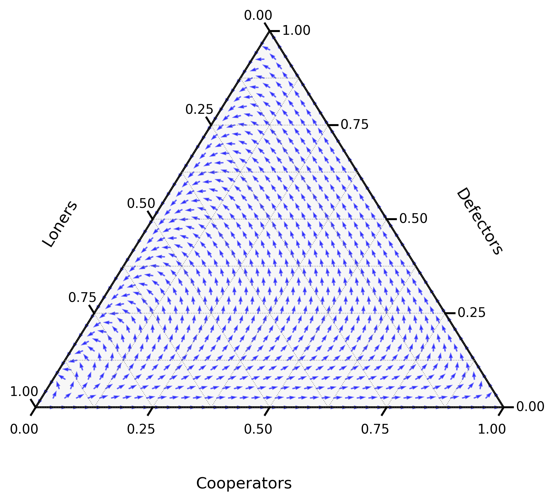
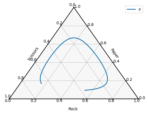
A simplex with the evolutionary trajectory of the underlying replicator dynamics equation — Figure 1:A diagram showing the direction of the derivative as given by (1) for $r=3$ and $\sigma=.6$ .

Strategies that do better than the average will increase in frequency; those that do worse will decline. This feedback mechanism drives the evolution of behaviour in the population, capturing the shifting fortunes of cooperators, defectors, and loners on campus.

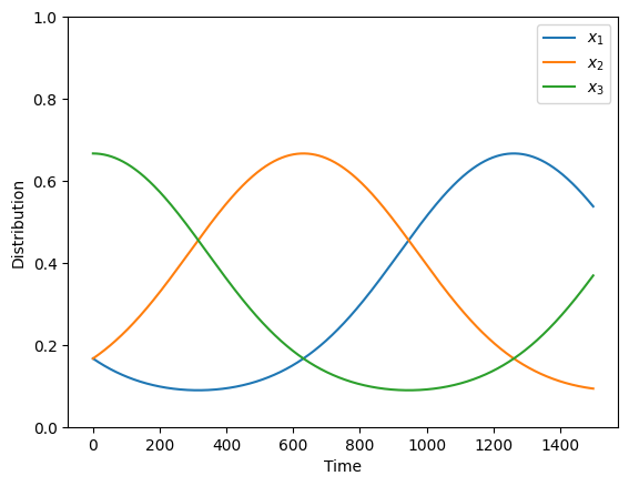
As we will see, this system often exhibits cyclical behaviour: when most students cooperate, defectors thrive; when defection becomes too common, students prefer to be loners; when clubs are small and rare, cooperation becomes appealing again. These cycles, and their stability, are precisely what replicator dynamics helps us understand.

Theory¶

Definition: Replicator Dynamics Equation¶

Consider a population with $N$ types of individuals. Let $x_i$ denote the proportion of individuals of type $i$ , so that $\sum_{i=1}^N x_i = 1$ .

Suppose the fitness of an individual of type $i$ depends on the state of the entire population, through a population-dependent fitness function $f_i(x)$ .

The replicator dynamics equation is given by:

\frac{dx_i}{dt} = x_i(f_i(x) - \phi) \quad \text{for all } i

(2)

where the average population fitness $\phi$ is defined as:

\phi = \sum_{i=1}^N x_i f_i(x)

(3)

This equation describes the change in frequency of each type as proportional to how much better (or worse) its fitness is compared to the population average.

Example: The common good game¶

In the common good game around coffee clubs the replicator dynamics equation can be written as:

\begin{align*} \dot{x}_c &= x_c\left(\frac{rx_c}{x_c + x_d} - 1 - \phi\right)\\ \dot{x}_d &= x_d\left(\frac{rx_c}{x_c + x_d} - \phi\right)\\ \dot{x}_l &= x_l\left(\sigma - \phi\right)\\ \end{align*}

(4)

where:

\begin{align*} \phi &= x_c \left(\frac{rx_c}{x_c + x_d} - 1\right) + x_d \left(\frac{rx_c}{x_c + x_d}\right) + x_l\sigma\\ &= \frac{rx_c^2}{x_c + x_d} - x_c + \frac{rx_cx_d}{x_c + x_d} + x_l\sigma\\ &= \frac{rx_c^2 - x_c(x_c+x_d) + rx_cx_d + x_l\sigma(x_c + x_d)}{x_c + x_d}\\ &= \frac{rx_c(x_c + x_d) - x_c(x_c+x_d) + x_l\sigma(x_c + x_d)}{x_c + x_d}\\ &= \frac{(x_c + x_d)\left(rx_c - x_c + x_l\sigma\right)}{x_c + x_d}\\ &= x_c(r - 1) + x_l\sigma \end{align*}

(5)

Definition: Stable Population¶

For a given population game with $N$ types of individuals and fitness functions $f_i$ a stable population $\tilde x$ is one for which $\dot x_i=0$ for all $i$ .

For a stable population $\tilde x_i$ :

\dot{x}_i = \tilde x_i(f_i(\tilde x_i) - \phi) = 0

(6)

so either: $\tilde x_i=0$ or $f_i(\tilde x_i) = \phi$ .

Example: No interior point stable population in the common goods game¶

For the common good game around coffee clubs we have some immediate stable populations:

$x=(x_c, x_d, x_l) = (0, 0, 1)$ : indeed $\dot x_c = \dot x_d = 0$ so that $\phi=\sigma$ and so $\dot x_l = 0$ .
$x=(x_c, x_d, x_l) = (0, 1, 0)$ : indeed $\dot x_c = \dot x_l = 0$ so that $\phi=f_d(x)=0$ and so $\dot x_d = 0$ .
$x=(x_c, x_d, x_l) = (1, 0, 0)$ : indeed $\dot x_d = \dot x_l = 0$ so that $\phi=f_c(x)=r-1$ and so $\dot x_c = 0$ .

A question remains, is there a point in the interior of the simplex of Figure 1 that is stable? Such a point has $x_c>0$ , $x_d>0$ and $x_l > 0$ which implies:

f_c(x) = f_d(x) = f_l(x)

(7)

This is not possible as: $f_c(x) = f_d(x) - 1$ for all $x$ .

Definition: Fitness of a strategy in a population¶

In a population with $N$ types let $f(y, x)$ denote the fitness of an individual playing strategy $y$ in a population $x$ :

f(y, x) = \sum_{i=1}^Ny_if_i(x)

(8)

Example: A new student in the Common Goods Game¶

For the common good game if we consider a stable population $x=(0, 1, 0)$ where everyone is defecting and assume that a new student enters planning to cooperate 50% of the time and defect 50% of the time, their fitness is given by:

f((1/2, 1/2, 0), (0, 1, 0)) = 1/2 f_c(0, 1, 0) + 1/2f_d(0, 1, 0) = 1/2 \cdot (-1) + 1/2 \cdot 0 = -1/2

(9)

Definition: Post Entry Population¶

For a population with $N$ types of individuals Given a population $x \in \mathbb{R}^N_{[0, 1]}$ (with $\sum_{i=1}^Nx_i=1$ ), some $\epsilon>0$ and a strategy $y \in \mathbb{R}^N_{[0, 1]}$ (with $\sum_{i=1}^Ny_i=1$ ), the post entry population $x_{\epsilon}$ is given by:

x_{\epsilon} = x + \epsilon(y - x)

(10)

Example: Post Entry Population for the Common Goods Game¶

For the common good game if we consider the stable population $x=(0, 1, 0)$ where everyone is defecting and assume that a new student enters the population planning to cooperate with a coffee club 50% of the time and defect 50% of the time the post entry population will be:

x_{\epsilon} = (0, 1, 0) + \epsilon((1/2, 1/2, 0) - (0, 1, 0)) = (0, 1, 0) + (\epsilon/2, -\epsilon/2, 0) = (\epsilon / 2, 1 - \epsilon / 2, 0)

(11)

What is of interest in the field of evolutionary game theory is what happens to the post entry population: does this new student change the stability of the system or is the system going to go back to all students defecting? This is the question of evolutionary stability. The evolutionarily stable strategy (ESS), defined formally below, captures exactly this: a population is evolutionarily stable if residents always outperform any rare mutant. For pairwise interaction games the invasion condition reduces to a convenient algebraic characterisation, also developed below.

Definition: Pairwise Interaction Game¶

Given a population of $N$ types of individuals and a payoff matrix $M^{n\times n}$ a pairwise interaction game is a game where the fitness is $f_i(x)$ is given by:

f_i(x) = \sum_{j=1}^{N}x_jM_{ij}

(12)

This corresponds to a population where all individuals interact with all other individuals in the population and obtain a fitness given by the matrix $M$ .

Note that there is a linear algebraic equivalent to (12):

f = xM

(13)

and then:

\phi = x f

(14)

Example: The Hawk Dove Game¶

Consider a population of animals. These animals, when they interact, will always share their food. Due to a genetic mutation, some of these animals may act in an aggressive manner and not share their food. If two aggressive animals meet, they both compete and end up with no food. If an aggressive animal meets a sharing one, the aggressive one will take most of the food.

These interactions can be represented using the matrix $A$ :

M = \begin{pmatrix} 2 & 1\\ 3 & 0 \end{pmatrix}

(15)

In this scenario: what is the likely long-term effect of the genetic mutation?

Over time will:

The population resist the mutation and all the animals continue to share their food.
The population get taken over by the mutation and all animals become aggressive.
A mix of animals are present in the population: some act aggressively and some share.

To answer this question, we will model it as a pairwise interaction game with $x\in\mathbb{R}_{[0, 1]}^2$ representing the population distribution. In this case:

$x_1$ represents the proportion of the population that shares.
$x_2$ represents the proportion of the population that acts aggressively.

In this case, the replicator dynamics equation becomes:

\begin{align*} \frac{dx_1}{dt} &= x_1(2x_1 + x_2 - \phi) \\ \frac{dx_2}{dt} &= x_2(3x_1 - \phi) \end{align*}

(16)

\phi = x_1(2x_1 + x_2) + x_2(3x_1)

(17)

Note that $x_2 = 1 - x_1$ so for simplicity of notation we will only use $x$ to represent the proportion of the population that shares.

Thus we can write the single differential equation:

\begin{align*} \frac{dx}{dt} &= x (2x + (1 - x) - \phi)\\ &= x (2x + (1 - x) - x(2x + (1-x)) - (1 - x)(3x))\\ &= x (2x^2-3x+1)\\ &= x(x -1)(2x-1) \end{align*}

(18)

We see that there are 3 stable populations:

$x=0$ : No sharers
$x=1$ : Only sharers
$x=1/2$ : A mix of both sharers and aggressive individuals.

This differential equation can then be solved numerically, for example using Euler’s Method to show the evolution of

Let us do this with a step size $h=.1$ and an initial population of $x=3/5$ :

Recall, we use the update rule:

x_{n+1} = x_n + h \cdot f(x_n)

(19)

to give Table 1.

Table 1:Step by step application of Euler’s method to the Hawk Dove game with step size $h=.1$ and $x_0=3/5$ .

$n$	$t_n$	$x_n$	$f(x_n)$	$x_{n+1}$
0	0.0	0.600	-0.048	0.595
1	0.1	0.595	-0.046	0.591
2	0.2	0.591	-0.044	0.586
3	0.3	0.586	-0.042	0.582
4	0.4	0.582	-0.040	0.578
5	0.5	0.578	-0.038	0.574
6	0.6	0.574	-0.036	0.571
7	0.7	0.571	-0.035	0.567
8	0.8	0.567	-0.033	0.564
9	0.9	0.564	-0.031	0.561
10	1.0	0.561	-0.030	0.558

If we repeat this with $x=2/5$ we obtain Table 2.

Table 2:Step by step application of Euler’s method to the Hawk Dove game with step size $h=.1$ and $x_0=2/5$ .

$n$	$t_n$	$x_n$	$f(x_n)$	$x_{n+1}$
0	0.0	0.400	0.048	0.405
1	0.1	0.405	0.046	0.409
2	0.2	0.409	0.044	0.414
3	0.3	0.414	0.042	0.418
4	0.4	0.418	0.040	0.422
5	0.5	0.422	0.038	0.426
6	0.6	0.426	0.036	0.429
7	0.7	0.429	0.035	0.433
8	0.8	0.433	0.033	0.436
9	0.9	0.436	0.031	0.439
10	1.0	0.439	0.030	0.442

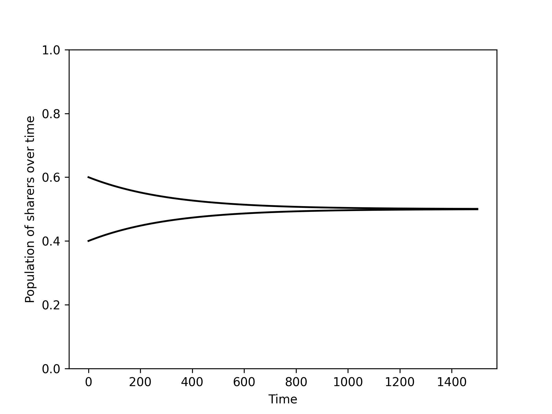
It looks the population is converging to the population which has a mix of both sharers and aggressive types: $x=1/2$ . Figure 2 confirms this.

A plot of two lines, one starting at 3/5 and the other at 2/5. The lines slowly converge to 1/2. — Figure 2:The numerical integration of the differential equation (18) with two different initial values of $x$ .

This indicates that $x=1/2$ is an evolutionary stable strategy. To confirm this we could apply the definition of an evolutionarily stable strategy directly; however, for pairwise interaction games there is a theoretic result that can be used instead. We first state the definition formally.

Definition: Evolutionarily Stable Strategy¶

A strategy $\sigma^*$ is an evolutionarily stable strategy (ESS) if there exists $\bar\epsilon > 0$ such that for all $\sigma' \neq \sigma^*$ and all $0 < \epsilon < \bar\epsilon$ ,

f\!\bigl(\sigma^*,\,(1-\epsilon)\sigma^* + \epsilon\sigma'\bigr) \;>\; f\!\bigl(\sigma',\,(1-\epsilon)\sigma^* + \epsilon\sigma'\bigr)

(20)

where $(1-\epsilon)\sigma^* + \epsilon\sigma'$ is the post-entry population: a population consisting mostly of residents with a small fraction $\epsilon$ of mutants.

The condition says that the resident strategy does strictly better than any rare mutant, so selection removes the mutant and the population returns to $\sigma^*$ . Letting $\epsilon \to 0$ gives $f(\sigma^*, \sigma^*) \geq f(\sigma', \sigma^*)$ for all $\sigma'$ , the Nash condition for symmetric games. Every ESS is therefore a symmetric Nash equilibrium, but not every Nash equilibrium is an ESS: ESS is a refinement that rules out equilibria vulnerable to invasion.

Theorem: Characterisation of ESS in two-player games¶

Let $\sigma^*$ be a strategy in a symmetric two-player game (so that $M_r=M_c^{\top}$ ). Then $\sigma^*$ is an evolutionarily stable strategy (ESS) if and only if, for all $\sigma \ne \sigma^*$ , one of the following conditions holds:

$f(\sigma^*, \sigma^*) > f(\sigma, \sigma^*)$
$f(\sigma^*, \sigma^*) = f(\sigma, \sigma^*)$ and
$f(\sigma^*, \sigma) > f(\sigma, \sigma)$

Conversely, if either of the above conditions holds for all $\sigma \ne \sigma^*$ , then $\sigma^*$ is an ESS in the corresponding population game.

Proof¶

Assume $\sigma^*$ is an ESS. Then, by definition, there exists $\varepsilon > 0$ such that for all $\sigma \ne \sigma^*$ and all $0 < \epsilon < \varepsilon$ , we have:

f(\sigma^*, \chi_\epsilon) > f(\sigma, \chi_\epsilon)

(21)

where $\chi_\epsilon = (1 - \epsilon)\sigma^* + \epsilon \sigma$ is the mixed population state. Substituting into the expected fitness, we obtain:

(1 - \epsilon) f(\sigma^*, \sigma^*) + \epsilon f(\sigma^*, \sigma) > (1 - \epsilon) f(\sigma, \sigma^*) + \epsilon f(\sigma, \sigma)

(22)

Rearranging, this inequality holds for all sufficiently small $\epsilon > 0$ if either:

$f(\sigma^*, \sigma^*) > f(\sigma, \sigma^*)$ (so the left-hand side is already greater); or
$f(\sigma^*, \sigma^*) = f(\sigma, \sigma^*)$ but $f(\sigma^*, \sigma) > f(\sigma, \sigma)$ , so the second-order term dominates as $\epsilon \to 0$ .

For the converse, suppose neither condition holds. Then either:

$f(\sigma^*, \sigma^*) < f(\sigma, \sigma^*)$ , so for small $\epsilon$ the inequality fails and $\sigma^*$ is not stable, or
$f(\sigma^*, \sigma^*) = f(\sigma, \sigma^*)$ and $f(\sigma^*, \sigma) \le f(\sigma, \sigma)$ , in which case the right-hand side is at least as large as the left for small $\epsilon$ , again contradicting stability.

Hence, the two conditions are necessary and sufficient for evolutionary stability.

This theorem gives us a practical method for identifying ESS:

Construct the associated symmetric two-player game.
Identify all symmetric Nash equilibria of the game.
For each symmetric Nash equilibrium, test the two conditions above.

Note that the first condition is very close to the condition for a strict Nash equilibrium, while the second adds a refinement that removes certain non-strict symmetric equilibria. This distinction is especially important when considering equilibria in strategies.

Example: Evolutionary stability in the Hawk-Dove game¶

Let us consider the Hawk-Dove game. The associated symmetric two-player game can be written in a general form. Let $v$ denote the value of the resource and $c$ the cost of conflict with $v < c$ .

Row player’s payoff matrix:

A = \begin{pmatrix} \frac{v-c}{2} & v \\ 0 & \frac{v}{2} \end{pmatrix}

(23)

Column player’s payoff matrix:

B = \begin{pmatrix} \frac{v-c}{2} & 0 \\ v & \frac{v}{2} \end{pmatrix}

(24)

To find symmetric Nash equilibria, we apply the support enumeration algorithm:

\begin{aligned} f(\sigma^*, H) &= f(\sigma^*, D) \\ q^* &= \frac{v}{c} \end{aligned}

(25)

This gives

\sigma^* = \left(\frac{v}{c}, 1 - \frac{v}{c}\right)

(26)

where individuals are aggressive with probability $\frac{v}{c}$ and share otherwise.

To determine whether this strategy is evolutionarily stable, we check the conditions of the characterisation theorem.

Since $f(\sigma^*, \sigma^*) = f(\sigma^*, \text{Aggressive}) = f(\sigma^*, \text{Sharing})$ , the first condition does not hold. We must therefore verify the second condition:

f(\sigma^*, \sigma) > f(\sigma, \sigma)

(27)

Let $\sigma = (\omega, 1 - \omega)$ be an arbitrary strategy. Then:

f(\sigma^*, \sigma) = \frac{v}{c} \cdot \omega \cdot \frac{v - c}{2} + \frac{v}{c} \cdot (1 - \omega) \cdot v + \left(1 - \frac{v}{c} \right) \cdot (1 - \omega) \cdot \frac{v}{2}

(28)

f(\sigma, \sigma) = \omega^2 \cdot \frac{v - c}{2} + \omega(1 - \omega) \cdot v + (1 - \omega)^2 \cdot \frac{v}{2}

(29)

Subtracting the two expressions gives:

\begin{align*} f(\sigma^*, \sigma) - f(\sigma, \sigma) \\ &= \frac{c}{2} \left( \frac{v}{c} - \omega \right)^2 > 0 \end{align*}

(30)

This inequality is strictly satisfied for all $\omega \ne \frac{v}{c}$ , so the second condition holds and $\sigma^*$ is an evolutionarily stable strategy.

Definition: Replicator Mutator Dynamics Equation¶

An extension of the replicator equation is to allow for mutation. In this setting, reproduction is imperfect: individuals of a given type can give rise to individuals of another type.

This process is represented by a matrix $Q$ , where $Q_{ij}$ denotes the probability that an individual of type $j$ is produced by an individual of type $i$ .

In this case, the replicator dynamics equation can be modified to yield the replicator-mutation equation:

\frac{dx_i}{dt} = \sum_{j=1}^N x_j f_j Q_{ji} - x_i \phi \quad \text{for all } i

(31)

Example: The Replicator Mutator Dynamics Equation for the Hawk Dove Game¶

Let there be a 10% chance that aggressive individuals will produce sharing ones in which case the matrix $Q$ is given by:

Q = \begin{pmatrix} 1 & 0\\ 1 / 10 & 9 / 10 \end{pmatrix}

(32)

Example: Recovering the Replicator Dynamics Equation from the Replicator Mutator Dynamics Equation¶

Show that when $Q=I_N$ (the identity matrix of size $N$ ) then the replicator dynamics equation corresponds to the replicator dynamics equation.

The replicator-mutation equation is:

\frac{dx_i}{dt} = \sum_{j=1}^N x_j f_j Q_{ji} - x_i \phi \quad \text{for all } i

(33)

As $Q = I_N$ :

Q_{ij} = \begin{cases} 1 & \text{if } i = j \\ 0 & \text{otherwise} \end{cases}

(34)

This gives:

\begin{align*} \frac{dx_i}{dt} &= x_i f_i Q_{ii} - x_i \phi \quad \text{for all } i && Q_{ij} = 0 \text{ for all } i \ne j \\ &= x_i f_i - x_i \phi \quad \text{for all } i && Q_{ii} = 1 \\ &= x_i (f_i - \phi) \quad \text{for all } i \end{align*}

(35)

Definition: Asymmetric Replicator Dynamics Equation¶

A further extension of the replicator dynamics framework accounts for populations divided into two distinct subsets. Individuals in the first population are one of $M$ possible types, while those in the second population are one of $N$ possible types.

This setting arises naturally in asymmetric games, where the roles of the players differ and the strategy sets need not be the same (i.e., $M \ne N$ ). In such cases, the standard replicator equation does not apply directly.

The asymmetric replicator dynamics equations describe the evolution of strategy distributions $x$ and $y$ in each population:

\frac{dx_i}{dt} = x_i\left((f_x)_i - \phi_x\right) \quad \text{for all } 1 \leq i \leq M

(36)

\frac{dy_j}{dt} = y_j\left((f_y)_j - \phi_y\right) \quad \text{for all } 1 \leq j \leq N

(37)

Here:

$(f_x)_i$ and $(f_y)_j$ are the expected fitnesses of type $i$ and $j$ in each population respectively,
$\phi_x$ and $\phi_y$ denote the average fitnesses in the respective populations.

Example: Tennis Serve and Return¶

In tennis, serving and receiving form an asymmetric interaction. The server (row player) chooses one of two serves, while the receiver (column player) chooses one of three possible return strategies.

The server can deliver a power or spin serve. The receiver can either prepare for power, cover a wide spin, or take an early aggressive position.

This leads to an asymmetric game where the server has 2 strategies and the receiver has 3. The game matrices are:

M_r = \begin{pmatrix} 3 & 1 & 2 \\ 4 & 2 & 1 \end{pmatrix}

(38)

M_c = \begin{pmatrix} 1 & 3 & 2 \\ 0 & 2 & 4 \end{pmatrix}

(39)

These matrices are based on the following assumptions:

If the server uses a power serve ( $r_1$ ) and the receiver prepares for it ( $c_1$ ), the server has some success (payoff 3), but the receiver also does reasonably well (payoff 1).
If the server tries spin ( $r_2$ ) and the receiver is covering for it ( $c_2$ ), the payoff is more balanced (2 for each).
A mismatch, such as a power serve into a receiver expecting spin ( $r_1$ vs $c_2$ ), favors the server more (payoff 1 vs 3).
Conversely, if the receiver takes an early position and guesses right against spin ( $r_2$ vs $c_3$ ), they gain a big advantage (payoff 1 vs 4).

Let $x = (x_1, x_2)$ be the strategy distribution of the server and $y = (y_1, y_2, y_3)$ that of the receiver. The asymmetric replicator dynamics for this game are:

\frac{dx_i}{dt} = x_i\left((A y)_i - x^\top A y\right) \quad \text{for } 1 \leq i \leq 2

(40)

\frac{dy_j}{dt} = y_j\left((x^\top B)_j - x^\top B y\right) \quad \text{for } 1\leq j \leq 3

(41)

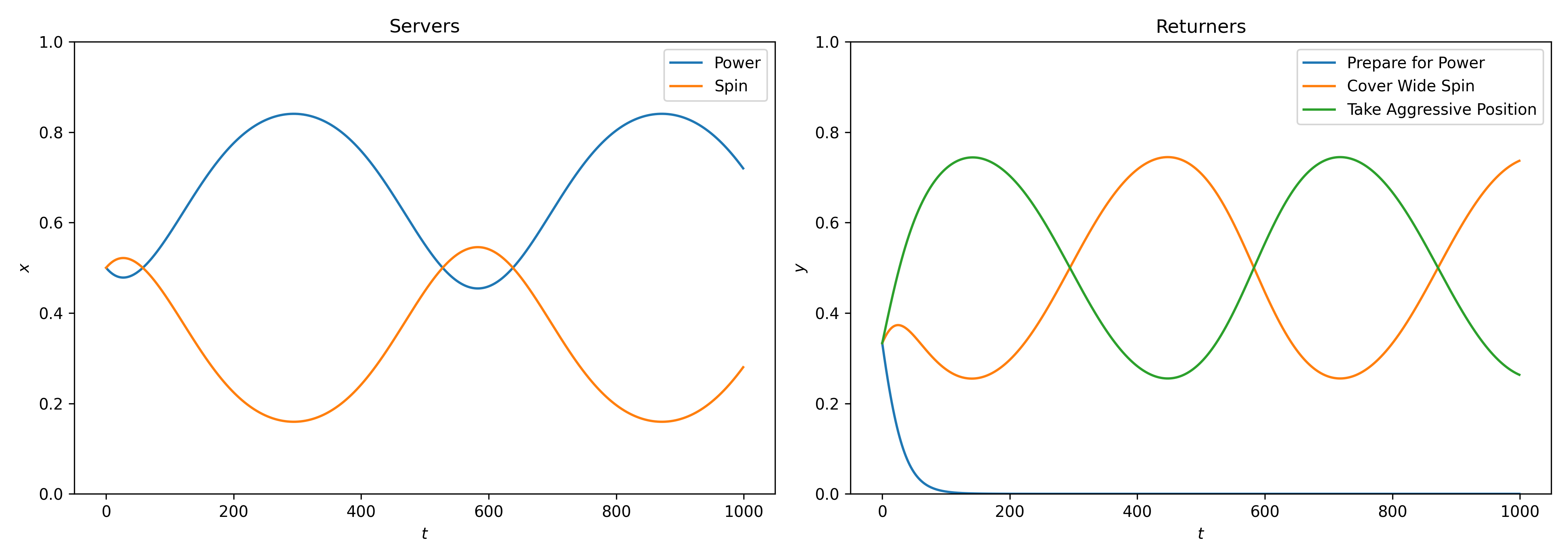
Figure 3 shows the numerical solutions of these differential equations over time.

Preparing for Power quickly dies out as a strategy;
There is a cycle with the server changing between power and spin while the returner cycles between preparing for spin and taking an aggressive position.

Two plots showing the numerical solutions of the asymmetric replicator dynamics equation — Figure 3:Numerical solutions to the asymmetric replicator dynamics equation. Preparing for power quickly dies out as a played strategy in the population. There is a cycle of the 2 remaining strategies for the returner and for the server although power remains the strategy player most often.

Exercises¶

Exercise 5

Throughout, the following game is considered:

Users of an online messaging platform can choose one of two incompatible apps: app $A$ or app $B$ .
The action set in this game is $\mathcal{A}=\{A, B\}$ .

Each user gains a base level of utility from being able to send messages at all. On top of this, their utility increases with the proportion of other users choosing the same app (since it becomes easier to contact friends).

Considering a population vector $x=(x_1,1 - x_1)$ where $x_1$ is the proportion of the population using app $A$ , the fitness functions are:

f_A(x)=1+2x_1, \qquad f_B(x)=1+2(1-x_1).

(46)

Give an interpretation for the fitness functions.
State the replicator dynamics equation for a population with two types.
Define a stable population for the replicator dynamics.
Define a post–entry population.
State the definition of an evolutionarily stable strategy (ESS).
Give the replicator dynamics equation for this game and obtain all stable populations.
For each of the following initial populations of $x\in\{(0.01, 0.99), (0.49,0.51), (0.99, 0.01)\}$ , calculate the first step of Euler’s method of numerical integration with a step size of $h=0.01$ .
In each case offer an interpretation in terms of evolutionary stability.
Now suppose that the strength of the coordination benefit is a parameter $a\neq 0$ , so that
$f_A(x)=1+a x_1, \qquad f_B(x)=1+a(1-x_1).$
(47)
Derive the replicator dynamics for general $a$ and determine for which values of $a$ the mixed population $x^\star=(\tfrac12,\tfrac12)$ is evolutionarily stable.
Justify your answer.

Programming¶

In Appendix: Numerical Integration, we introduce general programming approaches for numerically solving differential equations. These apply directly to the replicator dynamics equation. Here, we focus on tools specifically tailored to pairwise interaction games.

Solving symmetric replicator dynamics¶

The Nashpy library provides built-in functionality for solving the replicator dynamics equation in a pairwise interaction game.

Let us consider the classic Rock–Paper–Scissors game:

import nashpy as nash
import numpy as np

M_r = np.array([[0, 1, -1], [-1, 0, 1], [1, -1, 0]])
game = nash.Game(M_r)

We can compute the population trajectory from an initial distribution:

x0 = np.array([1 / 6, 1 / 6, 2 / 3])
timepoints = np.linspace(0, 10, 1500)
xs = game.replicator_dynamics(y0=x0, timepoints=timepoints).T
print(xs)

[[0.16666667 0.16611198 0.16555975 ... 0.53953201 0.53854678 0.53755904]
 [0.16666667 0.16722383 0.16778347 ... 0.09354312 0.09343612 0.09333053]
 [0.66666667 0.66666419 0.66665678 ... 0.36692487 0.36801711 0.36911043]]

To visualize the evolution of strategy frequencies over time:

import matplotlib.pyplot as plt

plt.figure()
plt.plot(xs.T)
plt.ylim(0, 1)
plt.legend(["$x_1$", "$x_2$", "$x_3$"])
plt.ylabel("Distribution")
plt.xlabel("Time")

Plotting a simplex with ternary¶

The ternary library Harper, 2019 allows for plotting trajectories on a simplex, ideal for representing three-component distributions that sum to one.

We can use it to plot the Rock–Paper–Scissors trajectory:

import ternary

figure, tax = ternary.figure(scale=1.0)
tax.boundary()
tax.gridlines(multiple=0.2, color="black")
# Plot the data
tax.plot(xs.T, linewidth=2.0, label="$x$")
tax.ticks(axis='lbr', multiple=0.2, linewidth=1, tick_formats="%.1f")
tax.legend()
tax.left_axis_label("Scissors")
tax.right_axis_label("Paper")
tax.bottom_axis_label("Rock")
tax.ax.axis('off')
tax.show()

Solving Asymmetric Replicator dynamics¶

The Nashpy library also supports numerical solutions for the asymmetric replicator dynamics equation.

M_r = np.array([[3, 1, 2], [4, 2, 1]])
M_c = np.array([[1, 3, 2], [0, 2, 4]])
game = nash.Game(M_r, M_c)

x0 = np.array([1/2, 1/2])
y0 = np.array([1/3, 1/3, 1/3])
timepoints = np.linspace(0, 20, 1000)

xs, ys = game.asymmetric_replicator_dynamics(x0=x0, y0=y0, timepoints=timepoints)
print(xs)

[[0.5        0.5       ]
 [0.49836507 0.50163493]
 [0.49679694 0.50320306]
 ...
 [0.72372346 0.27627654]
 [0.7218324  0.2781676 ]
 [0.7199282  0.2800718 ]]

The corresponding trajectory for the column player’s strategy distribution:

print(ys)

[[ 3.33333333e-01  3.33333333e-01  3.33333333e-01]
 [ 3.23391408e-01  3.36602736e-01  3.40005857e-01]
 [ 3.13590591e-01  3.39735869e-01  3.46673540e-01]
 ...
 [-1.06554178e-13  7.35381389e-01  2.64618611e-01]
 [-1.25688203e-13  7.36036679e-01  2.63963321e-01]
 [-1.40730981e-13  7.36668819e-01  2.63331181e-01]]

Notable Research¶

The original conceptual idea of an evolutionarily stable strategy (ESS) was formulated by Maynard Smith Maynard Smith & Price, 1973Maynard Smith, 1982. Although these works did not explicitly introduce the replicator dynamics equation, they were foundational in connecting game theory with evolutionary biology.

The first formal presentation of the replicator dynamics equation appeared in Taylor & Jonker, 1978, which directly built upon Maynard Smith’s ESS framework. This formulation was later extended to multi-player games in Palm, 1984, and to asymmetric populations in Accinelli & Carrera, 2011.

Several influential applications of replicator dynamics have since emerged. For example, Komarova et al., 2001 used replicator-mutator dynamics to model the spread of grammatical structures in language populations. In the context of cooperation, Hilbe et al., 2013 applied the model to study the evolution of reactive strategies, while Knight et al., 2024 recently demonstrated how extortionate strategies fail to persist under evolutionary pressure.

A particularly notable extension is found in Weitz et al., 2016, where the game itself changes dynamically depending on the population state. This approach is especially relevant in modelling the tragedy of the commons and other environmental feedback systems.

In Lv et al., 2023, a model similar to the one in Section: Motivating Example is examined using both replicator dynamics and a discrete population model. The latter is explored in detail in Chapter: Moran Process. Remarkably, the replicator dynamics equation emerges as the infinite-population limit of the discrete model, a connection rigorously established in Traulsen et al., 2005.

Conclusion¶

The replicator dynamics equation provides a powerful lens through which to study strategy evolution in large populations. By linking the fitness of strategies to their growth or decline in the population, it captures the essence of selection and adaptation.

Throughout this chapter, we explored how replicator dynamics:

arise naturally in settings like public goods provision (e.g., coffee clubs),
describe population change in terms of differential equations,
connect with the concept of evolutionarily stable strategies (ESS),
extend to incorporate mutation and asymmetry,
and can be simulated and visualized with numerical methods and tools.

From modelling simple two-strategy contests to rich three-strategy dynamics on a simplex, replicator dynamics offer an interpretable and analytically rich framework for evolutionary game theory. Table Table 3 gives a summary of the main concepts of this chapter.

Table 3:Summary of key concepts in replicator dynamics.

Concept	Description
Replicator Dynamics Equation	Models strategy frequency change based on relative fitness
Average Population Fitness ( $\phi$ )	Weighted average of individual fitnesses
Stable Population	A distribution where no strategy’s frequency changes over time
Evolutionarily Stable Strategy (ESS)	A stable strategy resistant to invasion by nearby alternatives
Post Entry Population	Perturbed population after a rare mutant enters
Replicator-Mutator Equation	Extension accounting for imperfect strategy transmission
Asymmetric Replicator Dynamics	Models evolution in multi-population or role-asymmetric settings
Pairwise Interaction Game	Fitness determined by payoffs in repeated pairwise interactions

Solutions¶

Solution to Exercise 1 #

For a population with two types the replicator dynamics reduce to a single equation. Writing $x = x_1$ and $x_2 = 1 - x$ ,

\dot x = x\bigl(f_1(x) - \phi\bigr), \qquad \phi = x f_1(x) + (1 - x) f_2(x),

(48)

so that

\dot x = x(1 - x)\bigl(f_1(x) - f_2(x)\bigr).

(49)

A population is stable when $\dot x = 0$ , that is when $x = 0$ , $x = 1$ , or $f_1(x) = f_2(x)$ . The two monomorphic populations $x = 0$ and $x = 1$ are always stable; any interior stable population solves $f_1(x) = f_2(x)$ .

Here $f_1 - f_2 = (x_1 - x_2) - (x_2 - 2x_1) = 5x - 2$ , which vanishes at $x = 2/5$ . The stable populations are $x \in \{0,\, 2/5,\, 1\}$ . Since $f_1 - f_2 < 0$ for $x < 2/5$ and $f_1 - f_2 > 0$ for $x > 2/5$ , the flow moves away from $2/5$ towards the nearer endpoint: the interior population is unstable and the two monomorphic populations are evolutionarily stable.
Here $f_1 = x_2(x_1 - 1) = -(1 - x)^2$ and $f_2 = 3/2 - 2x$ , so $f_1 - f_2 = -x^2 + 4x - 5/2$ . The only root in $[0, 1]$ is $x = 2 - \sqrt{6}/2 \approx 0.775$ (the other root exceeds 1). The stable populations are $x \in \{0,\, 2 - \sqrt{6}/2,\, 1\}$ . The interior root is again unstable, since $f_1 - f_2$ increases through zero there and nearby states are pushed to an endpoint.
Here $f_1 - f_2 = x_1^2 - x_2^2 = x_1 - x_2 = 2x - 1$ , which vanishes at $x = 1/2$ . The stable populations are $x \in \{0,\, 1/2,\, 1\}$ , with the interior mixed population unstable and the two monomorphic populations stable.

In every case the interior stable population is a repellor and only the monomorphic populations survive perturbation. We confirm this by integrating the replicator dynamics from post-entry states either side of each interior population.

import numpy as np

def replicator_trajectory(f_1, f_2, initial_x, step_size=0.01, steps=2000):
    trajectory = [initial_x]
    x = initial_x
    for _ in range(steps):
        average_fitness = x * f_1(x) + (1 - x) * f_2(x)
        x = x + step_size * x * (f_1(x) - average_fitness)
        trajectory.append(x)
    return np.array(trajectory)

fitness_pairs = {
    1: (lambda x: x - (1 - x), lambda x: (1 - x) - 2 * x),
    2: (lambda x: x * (1 - x) - (1 - x), lambda x: (1 - x) - x + 1 / 2),
    3: (lambda x: x ** 2, lambda x: (1 - x) ** 2),
}
interior_population = {1: 2 / 5, 2: 2 - np.sqrt(6) / 2, 3: 1 / 2}
for part, (f_1, f_2) in fitness_pairs.items():
    from_below = replicator_trajectory(f_1, f_2, interior_population[part] - 0.02)[-1]
    from_above = replicator_trajectory(f_1, f_2, interior_population[part] + 0.02)[-1]
    print(f"part {part}: from below -> {from_below:.3f}, from above -> {from_above:.3f}")

part 1: from below -> 0.000, from above -> 1.000
part 2: from below -> 0.000, from above -> 1.000
part 3: from below -> 0.000, from above -> 1.000

Solution to Exercise 2 #

For a pairwise interaction game with two types the fitness functions are $f_1(x) = A_{11}x_1 + A_{12}x_2$ and $f_2(x) = A_{21}x_1 + A_{22}x_2$ . As in the previous solution the dynamics reduce to $\dot x = x(1 - x)(f_1 - f_2)$ with $x = x_1$ and

f_1 - f_2 = (A_{11} - A_{21})x + (A_{12} - A_{22})(1 - x).

(50)

For $A = \begin{pmatrix} 2 & 4 \\ 5 & 3 \end{pmatrix}$ we obtain $f_1 - f_2 = -3x + (1 - x) = 1 - 4x$ , which vanishes at $x = 1/4$ . The stable populations are $x \in \{0,\, 1/4,\, 1\}$ . Here $f_1 - f_2 > 0$ for $x < 1/4$ and $f_1 - f_2 < 0$ for $x > 1/4$ , so the flow moves towards the interior population: $x = 1/4$ is stable and the two monomorphic populations are unstable. This is an anti-coordination (Hawk-Dove) game.
For $A = \begin{pmatrix} 1 & 0 \\ 0 & 1 \end{pmatrix}$ we obtain $f_1 - f_2 = x - (1 - x) = 2x - 1$ , which vanishes at $x = 1/2$ . The stable populations are $x \in \{0,\, 1/2,\, 1\}$ . This is a coordination game: the interior population is unstable and the two monomorphic populations are stable.

Solution to Exercise 3 #

We apply the characterisation of ESS for symmetric two-player games. In each case we identify the symmetric Nash equilibria and test the two conditions.

Here $A = \begin{pmatrix} 2 & 4 \\ 5 & 1 \end{pmatrix}$ . Neither pure strategy is a symmetric equilibrium: against residents playing the first strategy a mutant playing the second earns $5 > 2$ , and against residents playing the second a mutant playing the first earns $4 > 1$ . The only symmetric equilibrium is the fully mixed $\sigma^* = (1/2, 1/2)$ , obtained from $f_1 - f_2 = (2 - 5)x + (4 - 1)(1 - x) = 3 - 6x = 0$ . Because $\sigma^*$ is fully mixed, $f(\sigma^*, \sigma^*) = f(\sigma, \sigma^*)$ for every $\sigma$ , so the first condition never holds and we test the second. A direct calculation gives $f(\sigma^*, \sigma) - f(\sigma, \sigma) = \tfrac{3}{2}(2x - 1)^2 > 0$ for all $\sigma \neq \sigma^*$ , so $\sigma^* = (1/2, 1/2)$ is the unique ESS. This is an anti-coordination game and $\sigma^*$ is the attractor of the replicator dynamics.
Here $A = \begin{pmatrix} 1 & 0 \\ 0 & 1 \end{pmatrix}$ is a coordination game. Both pure strategies are strict symmetric equilibria: against residents playing the first strategy a mutant playing the second earns $0 < 1$ , so the first condition holds strictly and $e_1 = (1, 0)$ is an ESS; by symmetry $e_2 = (0, 1)$ is an ESS. The mixed equilibrium $\sigma^* = (1/2, 1/2)$ , from $2x - 1 = 0$ , is not an ESS: here $f(\sigma^*, \sigma) - f(\sigma, \sigma) = -\tfrac{1}{2}(2x - 1)^2 < 0$ , so a mutant does strictly better against the perturbed population and invades. The evolutionarily stable strategies are the two pure conventions.

Solution to Exercise 4 #

Write $x$ for the proportion $\mu$ of LaTeX users, so the two fitness functions are $f_L(x) = \alpha + 2x$ and $f_W(x) = 1 + 2(1 - x)$ . The replicator dynamics for two types reduce to

\dot x = x(1 - x)\bigl(f_L(x) - f_W(x)\bigr) = x(1 - x)\bigl(\alpha - 3 + 4x\bigr).

(51)

The fixed points are $x = 0$ (everyone uses Word), $x = 1$ (everyone uses LaTeX), and the interior point $x^* = (3 - \alpha)/4$ , which lies in $(0, 1)$ precisely when $1 < \alpha < 3$ .

The coefficient of $x$ inside the bracket is positive, so $f_L - f_W$ is increasing: this is a coordination game and any interior fixed point is a repellor. Checking the endpoints:

all-LaTeX ( $x = 1$ ): a lone Word user among LaTeX users earns $f_W(1) = 1$ against $f_L(1) = \alpha + 2 > 1$ , so $x = 1$ is a strict equilibrium and an ESS for every $\alpha > 1$ ;
all-Word ( $x = 0$ ): a lone LaTeX user among Word users earns $f_L(0) = \alpha$ against $f_W(0) = 3$ , so $x = 0$ is a strict equilibrium, and hence an ESS, if and only if $\alpha < 3$ .

Therefore, if $1 < \alpha < 3$ both conventions are evolutionarily stable and the department locks in to whichever system already predominates; the interior mixture $x^* = (3 - \alpha)/4$ is unstable and separates the two basins of attraction. If $\alpha \geq 3$ the intrinsic advantage of LaTeX is large enough that all-Word ceases to be stable and LaTeX is the only evolutionarily stable convention.

Solution to Exercise 5 #

The fitness of an app user is made up of:

a base utility of using any messaging app at all;
an extra utility that increases with the proportion of users choosing the same app.

For app $A$ :

\begin{align*} f_A(x) \\ &= \underbrace{1}_{\text{base utility of using any app}} + \underbrace{2x_1}_{\text{extra utility from many friends using app }A} \end{align*}

(52)

For app $B$ :

\begin{align*} f_B(x) \\ &= \underbrace{1}_{\text{base utility of using any app}} + \underbrace{2(1-x_1)}_{\text{extra utility from many friends using app }B} \end{align*}

(53)

So users gain more by coordinating on the same app as their friends.

If $x_1$ is the proportion of the population using strategy 1 (here, app $A$ ), the replicator dynamics for a two type population is:

\begin{align*} \frac{dx_1}{dt} \\ &= x_1\bigl(f_1(x) - \phi(x)\bigr), \end{align*}

(54)

where the average fitness $\phi(x)$ is

\begin{align*} \phi(x) \\ &= x_1 f_1(x) + (1-x_1) f_2(x). \end{align*}

(55)

From Definition: Stable Population:

For a given population game with $N$ types of individuals and fitness functions $f_i$ a stable population $\tilde x$ is one for which $\dot x_i=0$ for all $i$ .

From Definition: Post Entry Population: For a population with $N$ types of individuals Given a population $x \in \mathbb{R}^N_{[0, 1]}$ (with $\sum_{i=1}^Nx_i=1$ ), some $\epsilon>0$ and a strategy $y \in \mathbb{R}^N_{[0, 1]}$ (with $\sum_{i=1}^Ny_i=1$ ), the post entry population $x_{\epsilon}$ is given by:

x_{\epsilon} = x + \epsilon(y - x)

(56)

From Definition: Evolutionarily Stable Strategy:

A strategy $\sigma^*$ is an evolutionarily stable strategy if there exists $\bar\epsilon > 0$ such that for all $\sigma' \neq \sigma^*$ and all $0 < \epsilon < \bar\epsilon$ ,

f\!\bigl(\sigma^*,\,(1-\epsilon)\sigma^* + \epsilon\sigma'\bigr) \;>\; f\!\bigl(\sigma',\,(1-\epsilon)\sigma^* + \epsilon\sigma'\bigr)

(57)

where $(1-\epsilon)\sigma^* + \epsilon\sigma'$ is the post-entry population.

We have
$f_A(x)=1+2x_1, \qquad f_B(x)=1+2(1-x_1).$
(58)

The average fitness is

\begin{aligned} \phi(x) &= x_1 f_A(x) + (1-x_1) f_B(x) \\ &= x_1(1+2x_1) + (1-x_1)\bigl(1+2(1-x_1)\bigr) \\ &= x_1 + 2x_1^2 + (1-x_1)(3-2x_1) \\ &= x_1 + 2x_1^2 + 3 - 5x_1 + 2x_1^2 \\ &= 3 - 4x_1 + 4x_1^2. \end{aligned}

(59)

The replicator dynamics is

\begin{aligned} \frac{dx_1}{dt} &= x_1\bigl(f_A(x) - \phi(x)\bigr) \\ &= x_1\bigl((1+2x_1) - (3 - 4x_1 + 4x_1^2)\bigr) \\ &= x_1(-2 + 6x_1 - 4x_1^2) \\ &= -2x_1(2x_1^2 - 3x_1 + 1) \\ &= -2x_1(2x_1 - 1)(x_1 - 1). \end{aligned}

(60)

The fixed points are the solutions of $\frac{dx_1}{dt}=0$ :

x_1 \in \{0,\tfrac12,1\}.

(61)

The above answers the question, below is some code to confirm:

import sympy as sym

x_1 = sym.Symbol("x_1")

f_A = 1 + 2 * x_1
f_B = 1 + 2 * (1 - x_1)
phi = x_1 * f_A + (1 - x_1) * f_B
sym.simplify(phi)

x_1_dash = x_1 * (f_A - phi)
sym.simplify(x_1_dash)

x_1_dash = x_1 * (f_A - phi)
sym.solveset(x_1_dash, x_1)

We use the replicator equation from Question 6:

\begin{align*} \dot x_1 &= \frac{dx_1}{dt} \\ &= -2x_1(2x_1 - 1)(x_1 - 1). \end{align*}

(62)

Euler’s method with step size $h=0.01$ gives

x_1^{(1)} = x_1^{(0)} + h\,\dot x_1\big|_{x_1^{(0)}}.

(63)

(a) Initial population $x=(0.01,0.99)$

Here $x_1^{(0)}=0.01$ :

\begin{aligned} \dot x_1\big|_{0.01} &= -2\cdot 0.01\cdot(2\cdot 0.01 - 1)\cdot(0.01 - 1) \\ &= -2\cdot 0.01\cdot(-0.98)\cdot(-0.99) \\ &\approx -0.019404. \end{aligned}

(64)

Thus

\begin{align*} x_1^{(1)} \\ &= 0.01 + 0.01(-0.019404) \approx 0.009806. \end{align*}

(65)

Interpretation:
The proportion of $A$ –users decreases further from 0.01 to about 0.0098. This shows that, starting near the pure $B$ population, the dynamics move even closer to $(0,1)$ , confirming that the all– $B$ population is evolutionarily stable in this model.

The above answers the question, here is some code to confirm the calculations.

h = 0.01
initial_x_1 = 0.01
initial_x_1 + h * x_1_dash.subs({x_1: initial_x_1})

(b) Initial population $x=(0.49,0.51)$

Here $x_1^{(0)}=0.49$ :

\begin{aligned} \dot x_1\big|_{0.49} &= -2\cdot 0.49\cdot(2\cdot 0.49 - 1)\cdot(0.49 - 1) \\ &= -2\cdot 0.49\cdot(-0.02)\cdot(-0.51) \\ &\approx -0.009996. \end{aligned}

(66)

\begin{align*} x_1^{(1)} \\ &= 0.49 + 0.01(-0.009996) \approx 0.489900. \end{align*}

(67)

Interpretation:
Starting slightly below the mixed state $(\tfrac12,\tfrac12)$ , the proportion of $A$ –users decreases further (from 0.49 to about 0.4899). A small perturbation away from the mixed state does not return; instead it is pushed further away. This indicates that the mixed state is not evolutionarily stable.

The above answers the question, here is some code to confirm the calculations.

h = 0.01
initial_x_1 = 0.49
initial_x_1 + h * x_1_dash.subs({x_1: initial_x_1})

Initial population $x=(0.99,0.01)$

Here $x_1^{(0)}=0.99$ :

\begin{aligned} \dot x_1\big|_{0.99} &= -2\cdot 0.99\cdot(2\cdot 0.99 - 1)\cdot(0.99 - 1) \\ &= -2\cdot 0.99\cdot(0.98)\cdot(-0.01) \\ &\approx 0.019404. \end{aligned}

(68)

Thus

\begin{align*} x_1^{(1)} \\ &= 0.99 + 0.01(0.019404) \approx 0.990194. \end{align*}

(69)

Interpretation:
The proportion of $A$ –users increases slightly from 0.99 to about 0.9902. Starting near the pure $A$ population, the dynamics move even closer to $(1,0)$ , showing that the all– $A$ population is also evolutionarily stable.

The above answers the question, here is some code to confirm the calculations.

h = 0.01
initial_x_1 = 0.99
initial_x_1 + h * x_1_dash.subs({x_1: initial_x_1})

Overall, the dynamics push the population towards one of the two pure coordination states, and away from the mixed state.

We now let the strength of the coordination benefit be a parameter $a\neq 0$ :
$f_A(x)=1+a x_1, \qquad f_B(x)=1+a(1-x_1).$
(70)

(a) Replicator dynamics for general $a$

The average fitness is

\begin{aligned} \phi(x) &= x_1 f_A(x) + (1-x_1) f_B(x) \\ &= x_1(1+a x_1) + (1-x_1)\bigl(1+a(1-x_1)\bigr) \\ &= 2a x_1^2 - 2a x_1 + a + 1. \end{aligned}

(71)

Then

\begin{aligned} f_A(x) - \phi(x) &= (1 + a x_1) - (2a x_1^2 - 2a x_1 + a + 1) \\ &= a(-2x_1^2 + 3x_1 - 1) \\ &= -a(2x_1-1)(x_1-1). \end{aligned}

(72)

Thus the replicator dynamics is

\begin{align*} \frac{dx_1}{dt} \\ &= x_1\bigl(f_A(x) - \phi(x)\bigr) \\ &= -a\,x_1(2x_1-1)(x_1-1). \end{align*}

(73)

The fixed points satisfy $\frac{dx_1}{dt}=0$ , so again

x_1 \in \{0,\tfrac12,1\}.

(74)

To determine stability, we can consider all potential post entry populations or we can equivalently examine the sign of $\dot x_1$ :

First let us consider the case $a>0$ :

For $0<x_1<\tfrac12$ :
$x_1>0$ , $2x_1-1<0$ , $x_1-1<0$ so
$-ax_1(2x_1-1)(x_1-1)<0$ .
Thus for the post entry population $x_1=1/2-\epsilon$ $x_1(t)$ decreases and the flow moves away from $x_1=\tfrac12$ towards $x_1=0$ .
For $\tfrac12<x_1<1$ :
$x_1>0$ , $2x_1-1>0$ , $x_1-1<0$ so
$-ax_1(2x_1-1)(x_1-1)>0$ .
Thus for the post entry population $x_1=1/2+\epsilon$ $x_1(t)$ increases and the flow moves away from $x_1=\tfrac12$ towards $x_1=1$ .

Hence:

$x_1=\tfrac12$ is unstable;
$x_1=0$ and $x_1=1$ are evolutionary stable.

Now let us consider the case $a<0$ :

For $0<x_1<\tfrac12$ :
$x_1>0$ , $2x_1-1<0$ , $x_1-1<0$ so
$-ax_1(2x_1-1)(x_1-1)>0$ .
Thus for the post entry population $x_1=1/2-\epsilon$ $x_1(t)$ increases and the flow moves towards $x_1=\tfrac12$ .
For $\tfrac12<x_1<1$ :
$x_1>0$ , $2x_1-1>0$ , $x_1-1<0$ so
$-ax_1(2x_1-1)(x_1-1)<0$ .
Thus for the post entry population $x_1=1/2+\epsilon$ $x_1(t)$ decreases and the flow moves towards $x_1=\tfrac12$ .

If $a=0$ the derivative is 0 and thus all populations are stable.

Hence:

$x_1=\tfrac12$ is evolutionary stable;
$x_1=0$ and $x_1=1$ are unstable.

So $x^*=(1/2, 1/2)$ is an evolutionary stable strategy if and only if $a<0$ : the network effect is bad. There will only ever be an emergent population using both apps when the network effect is in fact negative.

The above answers the question. Here is some code to confirm the calculations and illustrate the sign of the derivative.

a = sym.Symbol("a")
f_A = 1 + a * x_1
f_B = 1 + a * (1 - x_1)
phi = x_1 * f_A + (1 - x_1) * f_B
sym.simplify(phi)

x_1_dash = x_1 * (f_A - phi)
sym.simplify(x_1_dash)

x_1_dash = x_1 * (f_A - phi)
sym.solveset(x_1_dash, x_1)

import matplotlib.pyplot as plt
import numpy as np

x_1 = sym.Symbol("x_1")

a = sym.Symbol("a")
f_A = 1 + a * x_1
f_B = 1 + a * (1 - x_1)
phi = x_1 * f_A + (1 - x_1) * f_B
x_1_dash = x_1 * (f_A - phi)
x_1_values = np.linspace(0, 1, 100)

plt.figure()
plt.plot(x_1_values, [x_1_dash.subs({x_1: x_value, a: -1}) for x_value in x_1_values], label="$a=-1$")
plt.plot(x_1_values, [x_1_dash.subs({x_1: x_value, a: -5}) for x_value in x_1_values], label="$a=-5$")
plt.plot(x_1_values, [x_1_dash.subs({x_1: x_value, a: 0}) for x_value in x_1_values], label="$a=0$")
plt.plot(x_1_values, [x_1_dash.subs({x_1: x_value, a: 1}) for x_value in x_1_values], label="$a=1$")
plt.plot(x_1_values, [x_1_dash.subs({x_1: x_value, a: 5}) for x_value in x_1_values], label="$a=5$")
plt.legend()
plt.xlabel("$x_1$")
plt.ylabel(r"$\frac{dx_1}{dt}$")

References¶

Harper, M. (2019). python-ternary: Ternary Plots in Python. Zenodo 10.5281/Zenodo.594435. 10.5281/zenodo.594435
Maynard Smith, J., & Price, G. R. (1973). The Logic of Animal Conflict. Nature, 246, 15–18. 10.1038/246015a0
Maynard Smith, J. (1982). Evolution and the Theory of Games. Cambridge University Press.
Taylor, P. D., & Jonker, L. B. (1978). Evolutionary stable strategies and game dynamics. Mathematical Biosciences, 40(1–2), 145–156.
Palm, G. (1984). Evolutionary stable strategies and game dynamics for n-person games. Journal of Mathematical Biology, 19, 329–334.
Accinelli, E., & Carrera, E. J. S. (2011). Evolutionarily stable strategies and replicator dynamics in asymmetric two-population games. In Dynamics, Games and Science I: DYNA 2008, in Honor of Maurı́cio Peixoto and David Rand, University of Minho, Braga, Portugal, September 8-12, 2008 (pp. 25–35). Springer.
Komarova, N. L., Niyogi, P., & Nowak, M. A. (2001). The evolutionary dynamics of grammar acquisition. Journal of Theoretical Biology, 209(1), 43–59.
Hilbe, C., Nowak, M. A., & Sigmund, K. (2013). Evolution of extortion in iterated prisoner’s dilemma games. Proceedings of the National Academy of Sciences, 110(17), 6913–6918.
Knight, V., Harper, M., Glynatsi, N. E., & Gillard, J. (2024). Recognising and evaluating the effectiveness of extortion in the Iterated Prisoner’s Dilemma. PloS One, 19(7), e0304641.
Weitz, J. S., Eksin, C., Paarporn, K., Brown, S. P., & Ratcliff, W. C. (2016). An oscillating tragedy of the commons in replicator dynamics with game-environment feedback. Proceedings of the National Academy of Sciences, 113(47), E7518–E7525.
Lv, S., Li, J., & Zhao, C. (2023). The evolution of cooperation in voluntary public goods game with shared-punishment. Chaos, Solitons & Fractals, 172, 113552.
Traulsen, A., Claussen, J. C., & Hauert, C. (2005). Coevolutionary dynamics: from finite to infinite populations. Physical Review Letters, 95(23), 238701.