Repeated Games

When the same game is played repeatedly, players can condition future behaviour on past actions, opening the door to cooperation that would be impossible in a one-shot interaction. This chapter shows how indefinite repetition can sustain cooperative outcomes, culminating in the Folk Theorem.

Motivating Example: Construction Contractors¶

Consider two local construction firms, Firm A and Firm B, who regularly bid on municipal infrastructure projects.

Each quarter, the city may announce a new contract for firms to bid on: a school, a road, or a public facility. These firms can choose to:

• Bid High (H): maintain high prices and sustain mutual profitability, or

• Bid Low (L): undercut the other firm to win the project outright.

If both firms bid high, they enjoy good margins and may take turns winning contracts. If one undercuts while the other bids high, the undercutter wins the project and earns a higher profit, at the cost of undermining trust. If both bid low, a price war ensues, shrinking profits for both.

However, the number of projects is not fixed in advance. After each bidding round, there is a probability $\delta \in (0, 1)$ that another project becomes available. Thus, the game is repeated probabilistically, with continuation probability $\delta$. The expected number of repetitions is $\frac{1}{1 - \delta}$.

Each firm chooses an action in each round:

• $H$: Bid High

• $L$: Bid Low

The one-shot payoff matrix is given by:

This is a classic example of a Prisoner’s Dilemma: short-term incentives tempt each player to defect (bid low), but long-term cooperation (bid high) could yield better payoffs.

The remainder of this chapter will explore:

• How cooperation can be sustained using history-dependent strategies.

• What conditions on $\delta$ allow for equilibrium cooperation.

• The formal statement and implications of the Folk Theorem.

Theory¶

Definition: repeated game¶

Given a two player game $(A,B)\in\mathbb{R}^{{m\times n}^2}$, referred to as a stage game, a $T$-stage repeated game is a game in which players play that stage game for $T>0$ repetitions. Players make decisions based on the full history of play over all the repetitions.

Example: Counting leaves in repeated games¶

Consider the following stage games and values of $T$. How many leaves would the extensive form representation of the repeated game have?

The initial play of the game has 4 outcomes (2 actions each). Each of these leads to 4 more in the second stage. Total: $4 \times 4 = 16$ leaves.

Same as (1): $4 \times 4 = 16$ leaves.

Definition: Strategies in a repeated game¶

A strategy for a player in a repeated game is a mapping from all possible histories of play to a probability distribution over the action set of the stage game.

Example: Validity of repeated game strategies¶

For the Coordination Game with $T=2$ determine whether the following strategy pairs are valid, and if so, what outcome they lead to.

1. Row player:

Column player:

Valid strategy pair. Outcome: $(3,2)$ (corresponds to $O_9$ in the extensive form).

2. Row player:

Column player:

Invalid: the row player does not define an action for history $(S, C)$.

3. Row player:

Column player:

Invalid: column player uses an invalid action $\alpha$.

4. Row player:

Column player:

Valid strategy pair. Outcome: $(5,5)$ (corresponds to $O_4$ in the extensive form).

Theorem: Subgame perfection of sequence of stage Nash profiles¶

For any repeated game, any sequence of stage Nash profiles gives the outcome of a subgame perfect Nash equilibrium.

Where by stage Nash profile we refer to a strategy profile that is a Nash Equilibrium in the stage game.

Proof¶

Fix a stage Nash profile for each period: in period $k$ every player $i$ plays the action $\tilde s^{(k)}_i$ of some Nash equilibrium of the stage game, regardless of the history of play. This is a well-defined strategy profile for the repeated game, and it is history-independent, so it prescribes a stage Nash profile in every subgame.

We show it is subgame perfect by backward induction on the period. Total payoffs are the (discounted) sum of the stage payoffs, so in the final period $T$ each player faces exactly the stage game; since $\tilde s^{(T)}$ is a stage Nash profile, no player can gain by deviating in period $T$. Suppose the prescribed continuation from period $k+1$ onwards is a Nash equilibrium of every subgame it initiates. In period $k$ a player’s total payoff is their period-$k$ stage payoff plus a continuation payoff that, because the strategies ignore history, does not depend on the period-$k$ action. Optimising therefore reduces to the stage game, in which $\tilde s^{(k)}$ is a Nash profile, so again no player can gain by deviating. By the one-shot deviation principle no player has any profitable deviation in any subgame, and the profile is subgame perfect.

Example¶

Consider the following stage game:

There are two Nash equilibria in action space for this stage game:

For $T=2$ we have 4 possible outcomes that correspond to the outcome of a subgame perfect Nash equilibria:

Importantly, not all subgame Nash equilibria outcomes are of the above form.

Reputation¶

In a repeated game it is possible for players to encode reputation and trust in their strategies.

Example: Reputation in a repeated game¶

Consider the following stage game with $T=2$:

Through inspection it is possible to verify that the following strategy pair is a Nash equilibrium.

For the row player:

For the column player:

This pair of strategies corresponds to the following scenario:

The row player plays $r_1$ and the column player plays $c_2$ in the first stage. The row player plays $r_2$ and the column player plays $c_3$ in the second stage.

Note that if the row player deviates and plays $r_2$ in the first stage, then the column player will play $c_1$ in the second stage.

If both players play these strategies, their utilities are: $(11, 4)$, which is better for both players than the utilities at any sequence of stage Nash equilibria in action space.

But is this a Nash equilibrium? To find out, we investigate whether either player has an incentive to deviate.

1. If the row player deviates, they would only be rational to do so in the first stage. If they did, they would gain 1 in that stage but lose 4 in the second stage. Thus they have no incentive to deviate.

2. If the column player deviates, they would only do so in the first stage and gain no utility.

Thus, this strategy pair is a Nash equilibrium and evidences how reputation can be built and cooperation can emerge from complex dynamics.

Definition: Infinitely Repeated Game with Discounting¶

Given a two player game $(A,B)\in\mathbb{R}^{{m\times n}^2}$, referred to as a stage game, an infinitely repeated game with discounting factor $\delta$ is a game in which players play that stage game an infinite amount of times and gain the following utility:

where $u(s_r(i), s_c(i))$ denotes the utility obtained in the stage game for actions $s_r(i)$ and $s_c(i)$ which are the actions given by strategies $s_r$ and $s_c$ at stage $i$.

Example:¶

Consider Motivating Example: Construction Contractors and assume Firm A plans to undercut at all contracts: bidding low. Firm B plans to start by cooperating (bidding high) but if Firm A ever undercuts then Firm B will undercut for all subsequent contracts.

and

Replacing the values from the stage game this gives:

Definition: Average utility¶

If we interpret $\delta$ as the probability of the repeated game not ending then the average length of the game is:

We can use this to define the average payoff per stage:

Example:¶

Consider 3 strategies for Motivating Example: Construction Contractors:

• $S_c$ Always cooperate: bid high on all contracts.

• $S_d$ Always defect: bid low on all contracts.

• $S_g$ Grudger: bid high until facing a low bid and then bid low for ever.

For $\delta \in (1/4, 3/4)$:

1. Obtain the 3 by 3 Normal form game using average utility.

2. Check if mutual cooperation is a Nash equilibrium for both games.

We construct the Normal Form game representation with the 3 strategies becoming the action space (as described in Mapping Extensive Form Games to Normal Form).

We see that if $S_c$ is played against $S_g$ then both players cooperate at each stage giving:

For $S_d$ and $S_c$ we have:

For $S_g$ and $S_d$ we repeat the calculations of Example: to obtain:

and

Using the action space ordered as: $\{S_c, S_d, S_g\}$ this gives:

The game is symmetric so:

For $\delta=1/4$ this gives:

The game is symmetric so:

We see that $s_c$ and $s_g$ are both dominated by $s_d$ thus mutual cooperation is not a Nash equilibrium.

For $\delta=3/4$ this gives:

The game is symmetric so:

We see that mutual cooperation now is a Nash equilibrium because $s_g$ is now a best response to $s_g$.

The fact that cooperation can be stable for a higher value of $\delta$ is in fact a theorem that holds in the general case.

We need one final definition to describe what we imply:

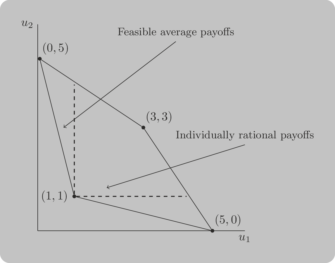
Definition of individually rational payoffs¶

Individually rational payoffs are average payoffs that exceed the stage game Nash equilibrium payoffs for both players.

As an example consider the plot corresponding to a repeated Prisoner’s Dilemma shown in Figure 3.

The feasible average payoffs correspond to the feasible payoffs in the stage game. The individually rational payoffs show the payoffs that are better for both players than the stage Nash equilibrium.

The following theorem states that we can choose a particular discount rate that for which there exists a subgame perfect Nash equilibrium that would give any individually rational payoff pair!

Theorem: Folk Theorem¶

Let $(u_1^*,u_2^*)$ be a pair of Nash equilibrium payoffs for a stage game. For every individually rational pair $(v_1,v_2)$ there exists $\bar \delta$ such that for all $1>\delta>\bar \delta>0$ there is a subgame perfect Nash equilibrium with payoffs $(v_1,v_2)$.

Proof¶

Let $(\sigma_1^*,\sigma_2^*)$ be the stage Nash profile that yields $(u_1^*,u_2^*)$. Now assume that playing $\bar\sigma_1\in\Delta \mathcal{A}_1$ and $\bar\sigma_2\in\Delta \mathcal{A}_2$ in every stage gives $(v_1,v_2)$ (an individual rational payoff pair).

Consider the following strategy:

“Begin by using $\bar \sigma_i$ and continue to use $\bar \sigma_i$ as long as both players use the agreed strategies. If any player deviates: use $\sigma_i^*$ for all future stages.”

We begin by proving that the above is a Nash equilibrium.

Without loss of generality if player 1 deviates to $\sigma_1'\in\Delta S_1$ such that $u_1(\sigma_1',\bar \sigma_2)>v_1$ in stage $k$ then:

Recalling that player 1 would receive $v_1$ in every stage with no deviation, the biggest gain to be made from deviating is if player 1 deviates in the first stage (all future gains are more heavily discounted). Thus if we can find $\bar\delta$ such that $\delta>\bar\delta$ implies that $U_1^{(1)}\leq \frac{v_1}{1-\delta}$ then player 1 has no incentive to deviate.

The most profitable one-stage deviation is the stage best response, so write $\hat u_1 = \max_{\sigma_1'} u_1(\sigma_1', \bar\sigma_2)$ for its payoff. As $(v_1, v_2)$ is individually rational we have $v_1 > u_1^*$, and the map $x \mapsto \tfrac{x - v_1}{x - u_1^*}$ is increasing for $x > v_1 > u_1^*$, so the binding threshold is the one for the best deviation. Taking $\bar\delta_1 = \frac{\hat u_1 - v_1}{\hat u_1 - u_1^*} \in (0, 1)$ ensures player 1 has no profitable deviation whenever $\delta > \bar\delta_1$. Repeating the argument for player 2 gives $\bar\delta_2$, and setting $\bar\delta = \max(\bar\delta_1, \bar\delta_2)$ shows that the prescribed strategy is a Nash equilibrium for all $\delta > \bar\delta$.

By construction this strategy is also a subgame perfect Nash equilibrium. Given any history both players will act in the same way and no player will have an incentive to deviate:

• If we consider a subgame just after any player has deviated from $\bar\sigma_i$ then both players use $\sigma_i^*$.

• If we consider a subgame just after no player has deviated from $\bar\sigma_i$ then both players continue to use $\bar\sigma_i$.

Exercises¶

Programming¶

Using Nashpy to generate repeated games¶

The Nashpy library has support for generating repeated games. Let us generate the repeated game obtained from the Prisoners Dilemma with $T=2$:

import nashpy.repeated_games

import nashpy as nash
import numpy as np

M_r = np.array([[3, 0], [5, 1]])
M_c = M_r.T
prisoners_dilemma = nash.Game(M_r, M_c)
repeated_pd = nash.repeated_games.obtain_repeated_game(game=prisoners_dilemma, repetitions=2)
print(repeated_pd)

Bi matrix game with payoff matrices:

Row player:
[[ 6.  6.  6. ...  3.  0.  0.]
 [ 6.  6.  6. ...  3.  0.  0.]
 [ 6.  6.  6. ...  3.  0.  0.]
 ...
 [ 8.  8.  8. ...  2.  6.  2.]
 [10. 10. 10. ...  1.  4.  1.]
 [10. 10. 10. ...  2.  6.  2.]]

Column player:
[[ 6.  6.  6. ...  8. 10. 10.]
 [ 6.  6.  6. ...  8. 10. 10.]
 [ 6.  6.  6. ...  8. 10. 10.]
 ...
 [ 3.  3.  3. ...  2.  1.  2.]
 [ 0.  0.  0. ...  6.  4.  6.]
 [ 0.  0.  0. ...  2.  1.  2.]]

We can directly obtain the action space of the row player for a given repeated game as a python generator:

strategies = nash.repeated_games.obtain_strategy_space(A=M_r, repetitions=2)
print(f"Number of row player strategies: {len(list(strategies))}")

Number of row player strategies: 32

To obtain the action space for the column player use A=M_c.T:

strategies = nash.repeated_games.obtain_strategy_space(A=M_c.T, repetitions=2)
print(f"Number of column player strategies: {len(list(strategies))}")

Number of column player strategies: 32

Notable research¶

The Folk Theorem presented in this chapter has a rich theoretical lineage. The foundational result is due to Friedman, 1971 (with a correction in Friedman, 1973), with the general formulation appearing in Fudenberg & Maskin, 1986. These results established the theoretical basis for understanding how cooperation can be sustained in long-run interactions.

Young, 1993 showed how social conventions and norms can emerge from adaptive play in repeated settings, providing an evolutionary foundation for Folk Theorem-type outcomes.

Conclusion¶

Repeated games introduce a rich strategic landscape where history matters and reputation can sustain cooperation. Unlike one-shot interactions, repeated games allow for long-term incentives to shape behaviour, often leading to outcomes that dominate those of stage game equilibria.

This chapter covered the formal definitions of repeated and infinitely repeated games, strategy spaces based on full histories, subgame perfection through sequences of Nash profiles, and the pivotal role of discounting. Through examples and the Folk Theorem, we saw how cooperation can emerge, even in environments like the Prisoner’s Dilemma, when players value the future sufficiently.

Table 1 summarises the key concepts.

Solutions¶