Cooperative Games
When players can form coalitions and make binding agreements, the key question
shifts from what strategy to play to how to share the resulting surplus fairly.
This chapter studies cooperative games through the characteristic function and
develops the Shapley value as a principled allocation scheme.
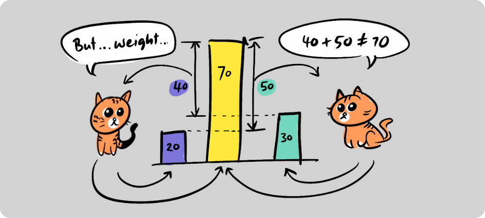
Figure 1: How much value does each player add to a cooperative effort? The marginal contribution
measures exactly this, and averaging it over every order of joining yields the
Shapley value, a principled way to share the surplus.
Motivating Example: Dividing the loot after a D&D battle ¶ After a climactic boss fight, a party of adventurers must divide a hoard of
The party includes:
Ren the fighter, who absorbed the dragon’s attacks.
Azel the wizard, who cast a decisive spell at the turning point.
Quinn the bard, who provided support and distracted the dragon
Each character played a crucial role, but in very different ways. How can they
Based on past encounters, the party has a sense of how much gold they might
{ Ren } = 0 \{\text{Ren}\} = 0 { Ren } = 0
{ Azel } = 0 \{\text{Azel}\} = 0 { Azel } = 0
{ Quinn } = 0 \{\text{Quinn}\} = 0 { Quinn } = 0
{ Ren , Azel } = 900 \{\text{Ren}, \text{Azel}\} = 900 { Ren , Azel } = 900
{ Ren , Quinn } = 400 \{\text{Ren}, \text{Quinn}\} = 400 { Ren , Quinn } = 400
{ Azel , Quinn } = 600 \{\text{Azel}, \text{Quinn}\} = 600 { Azel , Quinn } = 600
{ Ren , Azel , Quinn } = 1000 \{\text{Ren}, \text{Azel}, \text{Quinn}\} = 1000 { Ren , Azel , Quinn } = 1000
This is a classic example of a cooperative game , and understanding how to
Theory ¶ Definition: characteristic function game ¶ A characteristic function game G G G ( N , v ) (N, v) ( N , v ) N N N v : 2 [ N ] → R v: 2^{[N]} \to \mathbb{R} v : 2 [ N ] → R characteristic function which
Example: The characteristic function game of the D&D battle ¶ For the D&D battle N = 3 N = 3 N = 3 v v v
v ( c ) = { 0 if c = ∅ 0 if c = { Ren } 0 if c = { Azel } 0 if c = { Quinn } 900 if c = { Ren , Azel } 400 if c = { Ren , Quinn } 600 if c = { Azel , Quinn } 1000 if c = { Ren , Azel , Quinn } v(c) =
\begin{cases}
0 & \text{if } c = \emptyset \\
0 & \text{if } c = \{\text{Ren}\} \\
0 & \text{if } c = \{\text{Azel}\} \\
0 & \text{if } c = \{\text{Quinn}\} \\
900 & \text{if } c = \{\text{Ren}, \text{Azel}\} \\
400 & \text{if } c = \{\text{Ren}, \text{Quinn}\} \\
600 & \text{if } c = \{\text{Azel}, \text{Quinn}\} \\
1000 & \text{if } c = \{\text{Ren}, \text{Azel}, \text{Quinn}\}
\end{cases} v ( c ) = ⎩ ⎨ ⎧ 0 0 0 0 900 400 600 1000 if c = ∅ if c = { Ren } if c = { Azel } if c = { Quinn } if c = { Ren , Azel } if c = { Ren , Quinn } if c = { Azel , Quinn } if c = { Ren , Azel , Quinn } Definition: Monotone characteristic function game ¶ A characteristic function game G = ( N , v ) G = (N, v) G = ( N , v ) monotone if it satisfiesv ( C 2 ) ≥ v ( C 1 ) v(C_2) \geq v(C_1) v ( C 2 ) ≥ v ( C 1 ) C 1 ⊆ C 2 C_1 \subseteq C_2 C 1 ⊆ C 2
Example: The D&D battle is a monotone characteristic function game ¶ The function defined in (1)
v ( c ) = { 0 if c = ∅ 0 if c = { Ren } 0 if c = { Azel } 0 if c = { Quinn } 1100 if c = { Ren , Azel } 400 if c = { Ren , Quinn } 600 if c = { Azel , Quinn } 1000 if c = { Ren , Azel , Quinn } v(c) =
\begin{cases}
0 & \text{if } c = \emptyset \\
0 & \text{if } c = \{\text{Ren}\} \\
0 & \text{if } c = \{\text{Azel}\} \\
0 & \text{if } c = \{\text{Quinn}\} \\
1100 & \text{if } c = \{\text{Ren}, \text{Azel}\} \\
400 & \text{if } c = \{\text{Ren}, \text{Quinn}\} \\
600 & \text{if } c = \{\text{Azel}, \text{Quinn}\} \\
1000 & \text{if } c = \{\text{Ren}, \text{Azel}, \text{Quinn}\}
\end{cases} v ( c ) = ⎩ ⎨ ⎧ 0 0 0 0 1100 400 600 1000 if c = ∅ if c = { Ren } if c = { Azel } if c = { Quinn } if c = { Ren , Azel } if c = { Ren , Quinn } if c = { Azel , Quinn } if c = { Ren , Azel , Quinn } Indeed, Ren and Azel receive more without Quinn than with them, violating monotonicity.
Definition: superadditive characteristic function game ¶ A characteristic function game G = ( N , v ) G = (N, v) G = ( N , v ) superadditive if it satisfiesv ( C 1 ∪ C 2 ) ≥ v ( C 1 ) + v ( C 2 ) v(C_1 \cup C_2) \geq v(C_1) + v(C_2) v ( C 1 ∪ C 2 ) ≥ v ( C 1 ) + v ( C 2 ) C 1 ∩ C 2 = ∅ C_1 \cap C_2 = \emptyset C 1 ∩ C 2 = ∅
Example: The D&D battle is not a superadditive characteristic function game ¶ The function defined in (1)
v ( c ) = { 0 if c = ∅ 0 if c = { Ren } 700 if c = { Azel } 0 if c = { Quinn } 900 if c = { Ren , Azel } 400 if c = { Ren , Quinn } 600 if c = { Azel , Quinn } 1000 if c = { Ren , Azel , Quinn } v(c) =
\begin{cases}
0 & \text{if } c = \emptyset \\
0 & \text{if } c = \{\text{Ren}\} \\
700 & \text{if } c = \{\text{Azel}\} \\
0 & \text{if } c = \{\text{Quinn}\} \\
900 & \text{if } c = \{\text{Ren}, \text{Azel}\} \\
400 & \text{if } c = \{\text{Ren}, \text{Quinn}\} \\
600 & \text{if } c = \{\text{Azel}, \text{Quinn}\} \\
1000 & \text{if } c = \{\text{Ren}, \text{Azel}, \text{Quinn}\}
\end{cases} v ( c ) = ⎩ ⎨ ⎧ 0 0 700 0 900 400 600 1000 if c = ∅ if c = { Ren } if c = { Azel } if c = { Quinn } if c = { Ren , Azel } if c = { Ren , Quinn } if c = { Azel , Quinn } if c = { Ren , Azel , Quinn } Indeed:
v ( { Ren , Quinn } ) + v ( { Azel } ) = 400 + 700 = 1100 > 1000 = v ( { Ren , Azel , Quinn } ) v(\{\text{Ren}, \text{Quinn}\}) + v(\{\text{Azel}\}) = 400 + 700 = 1100 > 1000 = v(\{\text{Ren}, \text{Azel}, \text{Quinn}\}) v ({ Ren , Quinn }) + v ({ Azel }) = 400 + 700 = 1100 > 1000 = v ({ Ren , Azel , Quinn }) so the game violates superadditivity.
Definition: Payoff vector ¶ When we talk about a solution to a characteristic function game, we mean aλ ∈ R ≥ 0 N \lambda \in \mathbb{R}_{\geq 0}^N λ ∈ R ≥ 0 N λ \lambda λ
∑ i = 1 N λ i = v ( Ω ) \sum_{i=1}^N \lambda_i = v(\Omega) i = 1 ∑ N λ i = v ( Ω ) Example: A possible payoff vector: ¶ One possible payoff vector for (1)
λ = ( 200 , 350 , 450 ) \lambda = (200, 350, 450) λ = ( 200 , 350 , 450 ) This would seem unfair as Quinn gets 450 of the gold.
To find a “fair” distribution of the grand coalition we must
define what is meant by “fair”. We require four desirable properties:
Efficiency;
Null player;
Symmetry;
Additivity.
Definition: Efficiency ¶ Given a game G = ( N , v ) G = (N, v) G = ( N , v ) λ \lambda λ efficient if:
∑ i = 1 N λ i = v ( Ω ) \sum_{i=1}^N \lambda_i = v(\Omega) i = 1 ∑ N λ i = v ( Ω ) Example: An efficient Payoff Vector for the D&D Battle ¶ An efficient payoff vector is one that shares all 1,000 gold coins like the one
in (6)
Definition: Null Player Property ¶ Given a game G = ( N , v ) G = (N, v) G = ( N , v ) λ \lambda λ null player property if, for a player i i i
If v ( C ∪ i ) = v ( C ) v(C \cup i) = v(C) v ( C ∪ i ) = v ( C ) C ⊆ Ω C \subseteq \Omega C ⊆ Ω
Example: The Null Player Property in the D&D Battle ¶ In Motivating Example: Dividing the loot after a D&D battle
Definition: Symmetry Property ¶ Given a game G = ( N , v ) G = (N, v) G = ( N , v ) λ \lambda λ symmetry property if, for any pair of players i , j i, j i , j
If v ( C ∪ i ) = v ( C ∪ j ) v(C \cup i) = v(C \cup j) v ( C ∪ i ) = v ( C ∪ j ) C ⊆ Ω ∖ { i , j } C \subseteq \Omega \setminus \{i, j\} C ⊆ Ω ∖ { i , j }
λ i = λ j \lambda_i = \lambda_j λ i = λ j Example: The Symmetry Property in the D&D Battle ¶ In Motivating Example: Dividing the loot after a D&D battle
Definition: Additivity Property ¶ Given two games G 1 = ( N , v 1 ) G_1 = (N, v_1) G 1 = ( N , v 1 ) G 2 = ( N , v 2 ) G_2 = (N, v_2) G 2 = ( N , v 2 ) G + = ( N , v + ) G^+ = (N, v^+) G + = ( N , v + )
v + ( C ) = v 1 ( C ) + v 2 ( C ) for all C ⊆ Ω v^+(C) = v_1(C) + v_2(C) \quad \text{for all } C \subseteq \Omega v + ( C ) = v 1 ( C ) + v 2 ( C ) for all C ⊆ Ω A payoff vector λ \lambda λ additivity property if:
λ i ( G + ) = λ i ( G 1 ) + λ i ( G 2 ) \lambda_i^{(G^+)} = \lambda_i^{(G_1)} + \lambda_i^{(G_2)} λ i ( G + ) = λ i ( G 1 ) + λ i ( G 2 ) Example: The Additive Property in the D&D Battle ¶ In Motivating Example: Dividing the loot after a D&D battle
Definition: Predecessors ¶ Given a permutation π \pi π [ N ] [N] [ N ] predecessors of player i i i π \pi π S p i ( i ) S_pi(i) S p i ( i )
S π ( i ) = { j ∈ [ N ] ∣ π ( j ) < π ( i ) } S_\pi(i)=\{j \in [N] \mid \pi(j)<\pi(i)\} S π ( i ) = { j ∈ [ N ] ∣ π ( j ) < π ( i )} Example: The predecessors for the D&D Battle ¶ For Motivating Example: Dividing the loot after a D&D battle N = 3 N=3 N = 3 ( Ren , Azel , Quinn ) (\text{Ren}, \text{Azel}, \text{Quinn}) ( Ren , Azel , Quinn ) Table 1 3 ! = 6 3!=6 3 ! = 6 [ N ] [N] [ N ]
Table 1: The predecessors of each individual for each permutation
π \pi π S π ( 1 ) S_{\pi}(1) S π ( 1 ) S π ( 2 ) S_{\pi}(2) S π ( 2 ) S π ( 3 ) S_{\pi}(3) S π ( 3 ) ( 1 , 2 , 3 ) (1, 2, 3) ( 1 , 2 , 3 ) ∅ \emptyset ∅ { 1 } \{1\} { 1 } { 1 , 2 } \{1, 2\} { 1 , 2 } ( 1 , 3 , 2 ) (1, 3, 2) ( 1 , 3 , 2 ) ∅ \emptyset ∅ { 1 , 3 } \{1, 3\} { 1 , 3 } { 1 } \{1\} { 1 } ( 2 , 1 , 3 ) (2, 1, 3) ( 2 , 1 , 3 ) { 2 } \{2\} { 2 } ∅ \emptyset ∅ { 1 , 2 } \{1, 2\} { 1 , 2 } ( 2 , 3 , 1 ) (2, 3, 1) ( 2 , 3 , 1 ) { 2 , 3 } \{2, 3\} { 2 , 3 } ∅ \emptyset ∅ { 2 } \{2\} { 2 } ( 3 , 1 , 2 ) (3, 1, 2) ( 3 , 1 , 2 ) { 3 } \{3\} { 3 } { 1 , 3 } \{1, 3\} { 1 , 3 } ∅ \emptyset ∅ ( 3 , 2 , 1 ) (3, 2, 1) ( 3 , 2 , 1 ) { 2 , 3 } \{2, 3\} { 2 , 3 } { 3 } \{3\} { 3 } ∅ \emptyset ∅
Definition: Marginal Contribution ¶ Given a permutation π \pi π [ N ] [N] [ N ] marginal contribution of player
i i i π \pi π
Δ π G ( i ) = v ( S π ( i ) ∪ { i } ) − v ( S π ( i ) ) \Delta_\pi^G(i)=v(S_{\pi}(i)\cup \{i\})-v(S_{\pi}(i)) Δ π G ( i ) = v ( S π ( i ) ∪ { i }) − v ( S π ( i )) Example: Marginal Contributions in the D&D Battle ¶ For Motivating Example: Dividing the loot after a D&D battle ( Ren , Azel , Quinn ) (\text{Ren}, \text{Azel}, \text{Quinn}) ( Ren , Azel , Quinn ) N = 3 N = 3 N = 3 Table 2 Δ π G ( i ) \Delta_\pi^G(i) Δ π G ( i ) i i i π \pi π (1)
Table 2: Marginal contributions of each individual for each permutation
π \pi π Δ π G ( 1 ) \Delta_\pi^G(1) Δ π G ( 1 ) Δ π G ( 2 ) \Delta_\pi^G(2) Δ π G ( 2 ) Δ π G ( 3 ) \Delta_\pi^G(3) Δ π G ( 3 ) ( 1 , 2 , 3 ) (1, 2, 3) ( 1 , 2 , 3 ) 0 900 100 ( 1 , 3 , 2 ) (1, 3, 2) ( 1 , 3 , 2 ) 0 600 400 ( 2 , 1 , 3 ) (2, 1, 3) ( 2 , 1 , 3 ) 900 0 100 ( 2 , 3 , 1 ) (2, 3, 1) ( 2 , 3 , 1 ) 400 0 600 ( 3 , 1 , 2 ) (3, 1, 2) ( 3 , 1 , 2 ) 400 600 0 ( 3 , 2 , 1 ) (3, 2, 1) ( 3 , 2 , 1 ) 400 600 0
We are now ready to define the Shapley value for any cooperative game G = ( N , v ) G=(N,v) G = ( N , v )
Definition: Shapley Value ¶ Given a cooperative game G = ( N , v ) G=(N,v) G = ( N , v ) Shapley value of player i i i ϕ i ( G ) \phi_i(G) ϕ i ( G )
ϕ i ( G ) = 1 N ! ∑ π ∈ Π n Δ π G ( i ) \phi_i(G)=\frac{1}{N!}\sum_{\pi\in\Pi_n}\Delta_\pi^G(i) ϕ i ( G ) = N ! 1 π ∈ Π n ∑ Δ π G ( i ) Example: The Shapley Value for the D&D Battle ¶ For Motivating Example: Dividing the loot after a D&D battle Table 2
ϕ 1 = 0 + 0 + 900 + 400 + 400 + 400 6 = 350 ϕ 2 = 900 + 600 + 0 + 0 + 600 + 600 6 = 450 ϕ 3 = 100 + 400 + 100 + 600 + 0 + 0 6 = 200 \begin{align*}
\phi_1 &= \frac{0 + 0 + 900 + 400 + 400 + 400}{6} = 350\\
\phi_2 &= \frac{900 + 600 + 0 + 0 + 600 + 600}{6} = 450\\
\phi_3 &= \frac{100 + 400 + 100 + 600 + 0 + 0}{6} = 200\\
\end{align*} ϕ 1 ϕ 2 ϕ 3 = 6 0 + 0 + 900 + 400 + 400 + 400 = 350 = 6 900 + 600 + 0 + 0 + 600 + 600 = 450 = 6 100 + 400 + 100 + 600 + 0 + 0 = 200 Giving: ϕ = ( 350 , 450 , 200 ) \phi=(350, 450, 200) ϕ = ( 350 , 450 , 200 )
Exercises ¶ In statistics and machine learning, a linear model predicts a target
variable y y y x 1 , x 2 , … , x n x_1, x_2, \dots, x_n x 1 , x 2 , … , x n coefficient of determination , denoted R 2 R^2 R 2
In cooperative game theory, a characteristic function maps every coalition
(subset of players) to a value. In this exercise, we will interpret each feature
as a player, and define the value of a coalition to be the R 2 R^2 R 2
Suppose we are predicting a target variable y y y
y = c 1 x 1 + c 2 x 2 + c 3 x 3 y = c_1 x_1 + c_2 x_2 + c_3 x_3 y = c 1 x 1 + c 2 x 2 + c 3 x 3 Below are the R 2 R^2 R 2
Model R 2 R^2 R 2 y = c 1 x 1 y = c_1 x_1 y = c 1 x 1 0.122 y = c 2 x 2 y = c_2 x_2 y = c 2 x 2 0.097 y = c 3 x 3 y = c_3 x_3 y = c 3 x 3 0.551 y = c 1 x 1 + c 2 x 2 y = c_1 x_1 + c_2 x_2 y = c 1 x 1 + c 2 x 2 0.174 y = c 1 x 1 + c 3 x 3 y = c_1 x_1 + c_3 x_3 y = c 1 x 1 + c 3 x 3 0.581 y = c 2 x 2 + c 3 x 3 y = c_2 x_2 + c_3 x_3 y = c 2 x 2 + c 3 x 3 0.620 y = c 1 x 1 + c 2 x 2 + c 3 x 3 y = c_1 x_1 + c_2 x_2 + c_3 x_3 y = c 1 x 1 + c 2 x 2 + c 3 x 3 0.623
Define the characteristic function v ( S ) v(S) v ( S ) { x 1 , x 2 , x 3 } \{x_1, x_2, x_3\} { x 1 , x 2 , x 3 }
Compute the Shapley value for each feature with respect to the
characteristic function v v v
Interpret the result: Which feature contributes the most explanatory power?
Which contributes the least?
Consider the following two cooperative games defined on N = { 1 , 2 , 3 } N=\{1,2,3\} N = { 1 , 2 , 3 }
Game v a v_a v a
v a ( C ) = { 2 , if C = { 1 } 2 , if C = { 2 } 0 , otherwise v_a(C)=\begin{cases}
2, &\text{if }C=\{1\}\\
2, &\text{if }C=\{2\}\\
0, &\text{otherwise}
\end{cases} v a ( C ) = ⎩ ⎨ ⎧ 2 , 2 , 0 , if C = { 1 } if C = { 2 } otherwise Game v b v_b v b
v b ( C ) = { 1 , if C = { 1 , 3 } 1 , if C = { 2 , 3 } 3 , if C = { 1 , 2 , 3 } 0 , otherwise v_b(C)=\begin{cases}
1, &\text{if }C=\{1,3\}\\
1, &\text{if }C=\{2,3\}\\
3, &\text{if }C=\{1,2,3\}\\
0, &\text{otherwise}
\end{cases} v b ( C ) = ⎩ ⎨ ⎧ 1 , 1 , 3 , 0 , if C = { 1 , 3 } if C = { 2 , 3 } if C = { 1 , 2 , 3 } otherwise Verify that both games satisfy the symmetry property.
Obtain the Shapley value for v a v_a v a v b v_b v b
Construct the game ( v a + v b ) (v_a + v_b) ( v a + v b )
Verify that the Shapley value of ( v a + v b ) (v_a + v_b) ( v a + v b ) v a v_a v a v b v_b v b
Consider the cooperative game v v v N = { 1 , 2 , 3 } N=\{1,2,3\} N = { 1 , 2 , 3 }
v ( C ) = { 4 , if C = { 1 } 7 , if C = { 1 , 2 } 7 , if C = { 1 , 2 , 3 } 0 , otherwise v(C)=\begin{cases}
4, &\text{if }C=\{1\}\\
7, &\text{if }C=\{1,2\}\\
7, &\text{if }C=\{1,2,3\}\\
0, &\text{otherwise}
\end{cases} v ( C ) = ⎩ ⎨ ⎧ 4 , 7 , 7 , 0 , if C = { 1 } if C = { 1 , 2 } if C = { 1 , 2 , 3 } otherwise Identify any null players in this game.
Compute the marginal contributions of each player.
Calculate the Shapley value and confirm it respects the null player property.
Prove that the Shapley value satisfies the following properties:
Efficiency
Null player property
Symmetry
Additivity
Note that this does not prove uniqueness; that is, other vectors might satisfy these properties
(though in fact, the Shapley value is uniquely defined by them).
Programming ¶ The CoopGT library has functionality to verify properties of a characteristic
function game and also compute the Shapley value.
Here let us define a characteristic function and check if it is valid:
import coopgt.characteristic_function_properties


characteristic_function = {
    (): 0,
    (1,): 0,
    (2,): 0,
    (3,): 0,
    (1, 2): 900,
    (1,3): 400,
    (2, 3): 600,
    (1, 2, 3): 1000,
}
is_valid = coopgt.characteristic_function_properties.is_valid(
    characteristic_function=characteristic_function
)
print(f"Characteristic function valid? {is_valid}")
Characteristic function valid? True
Here we can check if it is monotone
is_monotone = coopgt.characteristic_function_properties.is_monotone(
    characteristic_function=characteristic_function
)
print(f"Characteristic function monotone? {is_monotone}")
Characteristic function monotone? True
Here we can check if it is
supperadditive
is_superadditive = coopgt.characteristic_function_properties.is_superadditive(
    characteristic_function=characteristic_function
)
print(f"Characteristic function superadditive? {is_superadditive}")
Characteristic function superadditive? True
Let us compute the Shapley value:
import coopgt.shapley_value

shapley_value = coopgt.shapley_value.calculate(
    characteristic_function=characteristic_function
)
print(f"Shapley value: {shapley_value}")
Shapley value: [350. 450. 200.]
Notable Research ¶ The Shapley value was first introduced by Shapley in Shapley & others, 1953 matching games .
In large games, the computational cost of calculating the Shapley value can be
prohibitive. While not necessarily intractable in the formal sense, as shown in
Deng & Papadimitriou, 1994 Castro et al. , 2009
One of the most impactful application areas of the Shapley value in recent years
has been in model explainability . As explored in
Exercise 2 Strumbelj & Kononenko, 2010 Jin et al. , 2022
Conclusion ¶ In this chapter, we introduced the theory of cooperative games , where groups
of players can form coalitions and share the resulting value. We focused on
characteristic function games , where the value of each coalition is known,
and explored how to fairly distribute this value using the Shapley value .
The four axioms (efficiency, null player, symmetry, and additivity) uniquely determine the Shapley value. We also saw applications to machine learning interpretability.
Table 3
Table 3: Summary of cooperative game concepts
Concept Description Characteristic function Maps each subset (coalition) of players to a real-valued payoff Monotonicity Adding players to a coalition cannot decrease its value Superadditivity The value of two disjoint coalitions is at most the value of their union Payoff vector A distribution of the total value among all players Marginal contribution The added value a player brings to a coalition Predecessors in permutation Players who appear before a given player in a permutation Shapley value The average marginal contribution: a unique, fair payoff satisfying four axioms
The Shapley value is the only payoff rule that satisfies efficiency , null
player , symmetry , and additivity , making it a principled way to fairly
divide rewards in cooperative settings.
Solutions ¶ Characteristic function v ( S ) v(S) v ( S )
Using the R 2 R^2 R 2 { x 1 , x 2 , x 3 } \{x_1, x_2, x_3\} { x 1 , x 2 , x 3 }
v ( ∅ ) = 0 , v ( { x 1 } ) = 0.122 , v ( { x 2 } ) = 0.097 , v ( { x 3 } ) = 0.551 v(\emptyset)=0,\quad v(\{x_1\})=0.122,\quad v(\{x_2\})=0.097,\quad v(\{x_3\})=0.551 v ( ∅ ) = 0 , v ({ x 1 }) = 0.122 , v ({ x 2 }) = 0.097 , v ({ x 3 }) = 0.551 v ( { x 1 , x 2 } ) = 0.174 , v ( { x 1 , x 3 } ) = 0.581 , v ( { x 2 , x 3 } ) = 0.620 v(\{x_1,x_2\})=0.174,\quad v(\{x_1,x_3\})=0.581,\quad v(\{x_2,x_3\})=0.620 v ({ x 1 , x 2 }) = 0.174 , v ({ x 1 , x 3 }) = 0.581 , v ({ x 2 , x 3 }) = 0.620 v ( { x 1 , x 2 , x 3 } ) = 0.623 v(\{x_1,x_2,x_3\})=0.623 v ({ x 1 , x 2 , x 3 }) = 0.623 Shapley value computation
We apply the formula with N = 3 N=3 N = 3
ϕ i ( v ) = ∑ S ⊆ N ∖ { i } ∣ S ∣ ! ( 2 − ∣ S ∣ ) ! 6 [ v ( S ∪ { i } ) − v ( S ) ] \phi_i(v)=\sum_{S\subseteq N\setminus\{i\}}\frac{|S|!(2-|S|)!}{6}\bigl[v(S\cup\{i\})-v(S)\bigr] ϕ i ( v ) = S ⊆ N ∖ { i } ∑ 6 ∣ S ∣ ! ( 2 − ∣ S ∣ )! [ v ( S ∪ { i }) − v ( S ) ] For x 1 x_1 x 1 (subsets S ⊆ { x 2 , x 3 } S\subseteq\{x_2,x_3\} S ⊆ { x 2 , x 3 }
S S S weight v ( S ∪ { x 1 } ) − v ( S ) v(S\cup\{x_1\})-v(S) v ( S ∪ { x 1 }) − v ( S ) ∅ \emptyset ∅ 2 / 6 2/6 2/6 0.122 − 0 = 0.122 0.122-0=0.122 0.122 − 0 = 0.122 { x 2 } \{x_2\} { x 2 } 1 / 6 1/6 1/6 0.174 − 0.097 = 0.077 0.174-0.097=0.077 0.174 − 0.097 = 0.077 { x 3 } \{x_3\} { x 3 } 1 / 6 1/6 1/6 0.581 − 0.551 = 0.030 0.581-0.551=0.030 0.581 − 0.551 = 0.030 { x 2 , x 3 } \{x_2,x_3\} { x 2 , x 3 } 2 / 6 2/6 2/6 0.623 − 0.620 = 0.003 0.623-0.620=0.003 0.623 − 0.620 = 0.003
Here ∣ S ∣ = 0 |S|=0 ∣ S ∣ = 0 ∣ S ∣ = 2 |S|=2 ∣ S ∣ = 2 0 ! 2 ! 6 = 2 6 \frac{0!\,2!}{6}=\frac{2}{6} 6 0 ! 2 ! = 6 2 ∣ S ∣ = 1 |S|=1 ∣ S ∣ = 1 1 ! 1 ! 6 = 1 6 \frac{1!\,1!}{6}=\frac{1}{6} 6 1 ! 1 ! = 6 1
ϕ x 1 = 2 ⋅ 0.122 + 1 ⋅ 0.077 + 1 ⋅ 0.030 + 2 ⋅ 0.003 6 = 0.357 6 ≈ 0.0595 \phi_{x_1}=\frac{2\cdot 0.122+1\cdot 0.077+1\cdot 0.030+2\cdot 0.003}{6}=\frac{0.357}{6}\approx 0.0595 ϕ x 1 = 6 2 ⋅ 0.122 + 1 ⋅ 0.077 + 1 ⋅ 0.030 + 2 ⋅ 0.003 = 6 0.357 ≈ 0.0595 For x 2 x_2 x 2 (subsets S ⊆ { x 1 , x 3 } S\subseteq\{x_1,x_3\} S ⊆ { x 1 , x 3 }
S S S weight v ( S ∪ { x 2 } ) − v ( S ) v(S\cup\{x_2\})-v(S) v ( S ∪ { x 2 }) − v ( S ) ∅ \emptyset ∅ 2 / 6 2/6 2/6 0.097 { x 1 } \{x_1\} { x 1 } 1 / 6 1/6 1/6 0.174 − 0.122 = 0.052 0.174-0.122=0.052 0.174 − 0.122 = 0.052 { x 3 } \{x_3\} { x 3 } 1 / 6 1/6 1/6 0.620 − 0.551 = 0.069 0.620-0.551=0.069 0.620 − 0.551 = 0.069 { x 1 , x 3 } \{x_1,x_3\} { x 1 , x 3 } 2 / 6 2/6 2/6 0.623 − 0.581 = 0.042 0.623-0.581=0.042 0.623 − 0.581 = 0.042
ϕ x 2 = 2 ⋅ 0.097 + 1 ⋅ 0.052 + 1 ⋅ 0.069 + 2 ⋅ 0.042 6 = 0.194 + 0.052 + 0.069 + 0.084 6 = 0.399 6 ≈ 0.0665 \phi_{x_2}=\frac{2\cdot 0.097+1\cdot 0.052+1\cdot 0.069+2\cdot 0.042}{6}=\frac{0.194+0.052+0.069+0.084}{6}=\frac{0.399}{6}\approx 0.0665 ϕ x 2 = 6 2 ⋅ 0.097 + 1 ⋅ 0.052 + 1 ⋅ 0.069 + 2 ⋅ 0.042 = 6 0.194 + 0.052 + 0.069 + 0.084 = 6 0.399 ≈ 0.0665 For x 3 x_3 x 3 (subsets S ⊆ { x 1 , x 2 } S\subseteq\{x_1,x_2\} S ⊆ { x 1 , x 2 }
S S S weight v ( S ∪ { x 3 } ) − v ( S ) v(S\cup\{x_3\})-v(S) v ( S ∪ { x 3 }) − v ( S ) ∅ \emptyset ∅ 2 / 6 2/6 2/6 0.551 { x 1 } \{x_1\} { x 1 } 1 / 6 1/6 1/6 0.581 − 0.122 = 0.459 0.581-0.122=0.459 0.581 − 0.122 = 0.459 { x 2 } \{x_2\} { x 2 } 1 / 6 1/6 1/6 0.620 − 0.097 = 0.523 0.620-0.097=0.523 0.620 − 0.097 = 0.523 { x 1 , x 2 } \{x_1,x_2\} { x 1 , x 2 } 2 / 6 2/6 2/6 0.623 − 0.174 = 0.449 0.623-0.174=0.449 0.623 − 0.174 = 0.449
ϕ x 3 = 2 ⋅ 0.551 + 1 ⋅ 0.459 + 1 ⋅ 0.523 + 2 ⋅ 0.449 6 = 1.102 + 0.459 + 0.523 + 0.898 6 = 2.982 6 ≈ 0.4970 \phi_{x_3}=\frac{2\cdot 0.551+1\cdot 0.459+1\cdot 0.523+2\cdot 0.449}{6}=\frac{1.102+0.459+0.523+0.898}{6}=\frac{2.982}{6}\approx 0.4970 ϕ x 3 = 6 2 ⋅ 0.551 + 1 ⋅ 0.459 + 1 ⋅ 0.523 + 2 ⋅ 0.449 = 6 1.102 + 0.459 + 0.523 + 0.898 = 6 2.982 ≈ 0.4970 Check : 0.0595 + 0.0665 + 0.4970 ≈ 0.623 = v ( { x 1 , x 2 , x 3 } ) 0.0595+0.0665+0.4970\approx 0.623=v(\{x_1,x_2,x_3\}) 0.0595 + 0.0665 + 0.4970 ≈ 0.623 = v ({ x 1 , x 2 , x 3 })
Interpretation
The Shapley values are approximately:
ϕ x 1 ≈ 0.060 , ϕ x 2 ≈ 0.067 , ϕ x 3 ≈ 0.497 \phi_{x_1}\approx 0.060,\quad\phi_{x_2}\approx 0.067,\quad\phi_{x_3}\approx 0.497 ϕ x 1 ≈ 0.060 , ϕ x 2 ≈ 0.067 , ϕ x 3 ≈ 0.497 Feature x 3 x_3 x 3 0.497 / 0.623 ≈ 80 % 0.497/0.623\approx 80\% 0.497/0.623 ≈ 80% R 2 R^2 R 2 x 1 x_1 x 1 x 2 x_2 x 2 x 1 x_1 x 1 x 2 x_2 x 2
import coopgt.shapley_value

v_linear = {
    (): 0,
    (1,): 0.122,
    (2,): 0.097,
    (3,): 0.551,
    (1, 2): 0.174,
    (1, 3): 0.581,
    (2, 3): 0.620,
    (1, 2, 3): 0.623,
}

shapley = coopgt.shapley_value.calculate(characteristic_function=v_linear)
print("Shapley values (x1, x2, x3):", shapley)
print(f"Sum: {sum(shapley):.3f} (should equal {v_linear[(1, 2, 3)]})")
Shapley values (x1, x2, x3): [0.0595 0.0665 0.497 ]
Sum: 0.623 (should equal 0.623)
Game v a v_a v a on N = { 1 , 2 , 3 } N=\{1,2,3\} N = { 1 , 2 , 3 }
v a ( C ) = { 2 , C = { 1 } 2 , C = { 2 } 0 , otherwise v_a(C)=\begin{cases}2, &C=\{1\}\\2, &C=\{2\}\\0, &\text{otherwise}\end{cases} v a ( C ) = ⎩ ⎨ ⎧ 2 , 2 , 0 , C = { 1 } C = { 2 } otherwise Game v b v_b v b on N = { 1 , 2 , 3 } N=\{1,2,3\} N = { 1 , 2 , 3 }
v b ( C ) = { 1 , C = { 1 , 3 } 1 , C = { 2 , 3 } 3 , C = { 1 , 2 , 3 } 0 , otherwise v_b(C)=\begin{cases}1, &C=\{1,3\}\\1, &C=\{2,3\}\\3, &C=\{1,2,3\}\\0, &\text{otherwise}\end{cases} v b ( C ) = ⎩ ⎨ ⎧ 1 , 1 , 3 , 0 , C = { 1 , 3 } C = { 2 , 3 } C = { 1 , 2 , 3 } otherwise Symmetry property
Recall the symmetry property: if v ( C ∪ { i } ) = v ( C ∪ { j } ) v(C\cup\{i\})=v(C\cup\{j\}) v ( C ∪ { i }) = v ( C ∪ { j }) C ⊆ Ω ∖ { i , j } C\subseteq\Omega\setminus\{i,j\} C ⊆ Ω ∖ { i , j } ϕ i = ϕ j \phi_i=\phi_j ϕ i = ϕ j
For v a v_a v a : Players 1 and 2 are symmetric. For every C ⊆ { 3 } C\subseteq\{3\} C ⊆ { 3 }
v a ( C ∪ { 1 } ) v_a(C\cup\{1\}) v a ( C ∪ { 1 }) C = ∅ C=\emptyset C = ∅ v a ( { 1 } ) = 2 v_a(\{1\})=2 v a ({ 1 }) = 2 C = { 3 } C=\{3\} C = { 3 } v a ( { 1 , 3 } ) = 0 v_a(\{1,3\})=0 v a ({ 1 , 3 }) = 0
v a ( C ∪ { 2 } ) v_a(C\cup\{2\}) v a ( C ∪ { 2 }) C = ∅ C=\emptyset C = ∅ v a ( { 2 } ) = 2 v_a(\{2\})=2 v a ({ 2 }) = 2 C = { 3 } C=\{3\} C = { 3 } v a ( { 2 , 3 } ) = 0 v_a(\{2,3\})=0 v a ({ 2 , 3 }) = 0
Since v a ( C ∪ { 1 } ) = v a ( C ∪ { 2 } ) v_a(C\cup\{1\})=v_a(C\cup\{2\}) v a ( C ∪ { 1 }) = v a ( C ∪ { 2 }) C ⊆ { 3 } C\subseteq\{3\} C ⊆ { 3 } v a v_a v a
v a v_a v a
For v b v_b v b : Players 1 and 2 are symmetric. For every C ⊆ { 3 } C\subseteq\{3\} C ⊆ { 3 }
C = ∅ C=\emptyset C = ∅ v b ( { 1 } ) = 0 = v b ( { 2 } ) v_b(\{1\})=0=v_b(\{2\}) v b ({ 1 }) = 0 = v b ({ 2 })
C = { 3 } C=\{3\} C = { 3 } v b ( { 1 , 3 } ) = 1 = v b ( { 2 , 3 } ) v_b(\{1,3\})=1=v_b(\{2,3\}) v b ({ 1 , 3 }) = 1 = v b ({ 2 , 3 })
v b v_b v b
Shapley values of v a v_a v a v b v_b v b
Shapley value of v a v_a v a :
Because v a v_a v a { 1 } \{1\} { 1 } { 2 } \{2\} { 2 }
π \pi π Δ π v a ( 1 ) \Delta^{v_a}_\pi(1) Δ π v a ( 1 ) Δ π v a ( 2 ) \Delta^{v_a}_\pi(2) Δ π v a ( 2 ) Δ π v a ( 3 ) \Delta^{v_a}_\pi(3) Δ π v a ( 3 ) ( 1 , 2 , 3 ) (1,2,3) ( 1 , 2 , 3 ) v a ( { 1 } ) = 2 v_a(\{1\})=2 v a ({ 1 }) = 2 v a ( { 1 , 2 } ) − v a ( { 1 } ) = − 2 v_a(\{1,2\})-v_a(\{1\})=-2 v a ({ 1 , 2 }) − v a ({ 1 }) = − 2 v a ( { 1 , 2 , 3 } ) − v a ( { 1 , 2 } ) = 0 v_a(\{1,2,3\})-v_a(\{1,2\})=0 v a ({ 1 , 2 , 3 }) − v a ({ 1 , 2 }) = 0 ( 1 , 3 , 2 ) (1,3,2) ( 1 , 3 , 2 ) 2 v a ( { 1 , 2 , 3 } ) − v a ( { 1 , 3 } ) = 0 v_a(\{1,2,3\})-v_a(\{1,3\})=0 v a ({ 1 , 2 , 3 }) − v a ({ 1 , 3 }) = 0 v a ( { 1 , 3 } ) − v a ( { 1 } ) = − 2 v_a(\{1,3\})-v_a(\{1\})=-2 v a ({ 1 , 3 }) − v a ({ 1 }) = − 2 ( 2 , 1 , 3 ) (2,1,3) ( 2 , 1 , 3 ) v a ( { 1 , 2 } ) − v a ( { 2 } ) = − 2 v_a(\{1,2\})-v_a(\{2\})=-2 v a ({ 1 , 2 }) − v a ({ 2 }) = − 2 v a ( { 2 } ) = 2 v_a(\{2\})=2 v a ({ 2 }) = 2 0 ( 2 , 3 , 1 ) (2,3,1) ( 2 , 3 , 1 ) v a ( { 1 , 2 , 3 } ) − v a ( { 2 , 3 } ) = 0 v_a(\{1,2,3\})-v_a(\{2,3\})=0 v a ({ 1 , 2 , 3 }) − v a ({ 2 , 3 }) = 0 2 v a ( { 2 , 3 } ) − v a ( { 2 } ) = − 2 v_a(\{2,3\})-v_a(\{2\})=-2 v a ({ 2 , 3 }) − v a ({ 2 }) = − 2 ( 3 , 1 , 2 ) (3,1,2) ( 3 , 1 , 2 ) v a ( { 1 , 3 } ) − v a ( { 3 } ) = 0 v_a(\{1,3\})-v_a(\{3\})=0 v a ({ 1 , 3 }) − v a ({ 3 }) = 0 v a ( { 1 , 2 , 3 } ) − v a ( { 1 , 3 } ) = 0 v_a(\{1,2,3\})-v_a(\{1,3\})=0 v a ({ 1 , 2 , 3 }) − v a ({ 1 , 3 }) = 0 v a ( { 3 } ) = 0 v_a(\{3\})=0 v a ({ 3 }) = 0 ( 3 , 2 , 1 ) (3,2,1) ( 3 , 2 , 1 ) v a ( { 1 , 2 , 3 } ) − v a ( { 2 , 3 } ) = 0 v_a(\{1,2,3\})-v_a(\{2,3\})=0 v a ({ 1 , 2 , 3 }) − v a ({ 2 , 3 }) = 0 v a ( { 2 , 3 } ) − v a ( { 3 } ) = 0 v_a(\{2,3\})-v_a(\{3\})=0 v a ({ 2 , 3 }) − v a ({ 3 }) = 0 0
ϕ 1 ( v a ) = 2 + 2 − 2 + 0 + 0 + 0 6 = 2 6 = 1 3 \phi_1(v_a)=\frac{2+2-2+0+0+0}{6}=\frac{2}{6}=\frac{1}{3} ϕ 1 ( v a ) = 6 2 + 2 − 2 + 0 + 0 + 0 = 6 2 = 3 1 ϕ 2 ( v a ) = − 2 + 0 + 2 + 2 + 0 + 0 6 = 2 6 = 1 3 \phi_2(v_a)=\frac{-2+0+2+2+0+0}{6}=\frac{2}{6}=\frac{1}{3} ϕ 2 ( v a ) = 6 − 2 + 0 + 2 + 2 + 0 + 0 = 6 2 = 3 1 ϕ 3 ( v a ) = 0 − 2 + 0 − 2 + 0 + 0 6 = − 4 6 = − 2 3 \phi_3(v_a)=\frac{0-2+0-2+0+0}{6}=\frac{-4}{6}=-\frac{2}{3} ϕ 3 ( v a ) = 6 0 − 2 + 0 − 2 + 0 + 0 = 6 − 4 = − 3 2 Check : 1 / 3 + 1 / 3 − 2 / 3 = 0 = v a ( { 1 , 2 , 3 } ) 1/3+1/3-2/3=0=v_a(\{1,2,3\}) 1/3 + 1/3 − 2/3 = 0 = v a ({ 1 , 2 , 3 })
Shapley value of v b v_b v b :
π \pi π Δ π v b ( 1 ) \Delta^{v_b}_\pi(1) Δ π v b ( 1 ) Δ π v b ( 2 ) \Delta^{v_b}_\pi(2) Δ π v b ( 2 ) Δ π v b ( 3 ) \Delta^{v_b}_\pi(3) Δ π v b ( 3 ) ( 1 , 2 , 3 ) (1,2,3) ( 1 , 2 , 3 ) 0 0 v b ( { 1 , 2 , 3 } ) − v b ( { 1 , 2 } ) = 3 v_b(\{1,2,3\})-v_b(\{1,2\})=3 v b ({ 1 , 2 , 3 }) − v b ({ 1 , 2 }) = 3 ( 1 , 3 , 2 ) (1,3,2) ( 1 , 3 , 2 ) 0 v b ( { 1 , 2 , 3 } ) − v b ( { 1 , 3 } ) = 2 v_b(\{1,2,3\})-v_b(\{1,3\})=2 v b ({ 1 , 2 , 3 }) − v b ({ 1 , 3 }) = 2 v b ( { 1 , 3 } ) − v b ( { 1 } ) = 1 v_b(\{1,3\})-v_b(\{1\})=1 v b ({ 1 , 3 }) − v b ({ 1 }) = 1 ( 2 , 1 , 3 ) (2,1,3) ( 2 , 1 , 3 ) 0 0 3 ( 2 , 3 , 1 ) (2,3,1) ( 2 , 3 , 1 ) v b ( { 1 , 2 , 3 } ) − v b ( { 2 , 3 } ) = 2 v_b(\{1,2,3\})-v_b(\{2,3\})=2 v b ({ 1 , 2 , 3 }) − v b ({ 2 , 3 }) = 2 0 v b ( { 2 , 3 } ) − v b ( { 2 } ) = 1 v_b(\{2,3\})-v_b(\{2\})=1 v b ({ 2 , 3 }) − v b ({ 2 }) = 1 ( 3 , 1 , 2 ) (3,1,2) ( 3 , 1 , 2 ) v b ( { 1 , 3 } ) − v b ( { 3 } ) = 1 v_b(\{1,3\})-v_b(\{3\})=1 v b ({ 1 , 3 }) − v b ({ 3 }) = 1 v b ( { 1 , 2 , 3 } ) − v b ( { 1 , 3 } ) = 2 v_b(\{1,2,3\})-v_b(\{1,3\})=2 v b ({ 1 , 2 , 3 }) − v b ({ 1 , 3 }) = 2 0 ( 3 , 2 , 1 ) (3,2,1) ( 3 , 2 , 1 ) v b ( { 1 , 2 , 3 } ) − v b ( { 2 , 3 } ) = 2 v_b(\{1,2,3\})-v_b(\{2,3\})=2 v b ({ 1 , 2 , 3 }) − v b ({ 2 , 3 }) = 2 v b ( { 2 , 3 } ) − v b ( { 3 } ) = 1 v_b(\{2,3\})-v_b(\{3\})=1 v b ({ 2 , 3 }) − v b ({ 3 }) = 1 0
ϕ 1 ( v b ) = 0 + 0 + 0 + 2 + 1 + 2 6 = 5 6 \phi_1(v_b)=\frac{0+0+0+2+1+2}{6}=\frac{5}{6} ϕ 1 ( v b ) = 6 0 + 0 + 0 + 2 + 1 + 2 = 6 5 ϕ 2 ( v b ) = 0 + 2 + 0 + 0 + 2 + 1 6 = 5 6 \phi_2(v_b)=\frac{0+2+0+0+2+1}{6}=\frac{5}{6} ϕ 2 ( v b ) = 6 0 + 2 + 0 + 0 + 2 + 1 = 6 5 ϕ 3 ( v b ) = 3 + 1 + 3 + 1 + 0 + 0 6 = 8 6 = 4 3 \phi_3(v_b)=\frac{3+1+3+1+0+0}{6}=\frac{8}{6}=\frac{4}{3} ϕ 3 ( v b ) = 6 3 + 1 + 3 + 1 + 0 + 0 = 6 8 = 3 4 Check : 5 / 6 + 5 / 6 + 4 / 3 = 5 / 6 + 5 / 6 + 8 / 6 = 18 / 6 = 3 = v b ( { 1 , 2 , 3 } ) 5/6+5/6+4/3=5/6+5/6+8/6=18/6=3=v_b(\{1,2,3\}) 5/6 + 5/6 + 4/3 = 5/6 + 5/6 + 8/6 = 18/6 = 3 = v b ({ 1 , 2 , 3 })
The game v + = v a + v b v^+ = v_a + v_b v + = v a + v b
v + ( C ) = v a ( C ) + v b ( C ) v^+(C)=v_a(C)+v_b(C) v + ( C ) = v a ( C ) + v b ( C ) C C C v a ( C ) v_a(C) v a ( C ) v b ( C ) v_b(C) v b ( C ) v + ( C ) v^+(C) v + ( C ) ∅ \emptyset ∅ 0 0 0 { 1 } \{1\} { 1 } 2 0 2 { 2 } \{2\} { 2 } 2 0 2 { 3 } \{3\} { 3 } 0 0 0 { 1 , 2 } \{1,2\} { 1 , 2 } 0 0 0 { 1 , 3 } \{1,3\} { 1 , 3 } 0 1 1 { 2 , 3 } \{2,3\} { 2 , 3 } 0 1 1 { 1 , 2 , 3 } \{1,2,3\} { 1 , 2 , 3 } 0 3 3
Using the Shapley formula for v + v^+ v +
ϕ 1 ( v + ) = ϕ 1 ( v a ) + ϕ 1 ( v b ) = 1 3 + 5 6 = 2 6 + 5 6 = 7 6 \phi_1(v^+)=\phi_1(v_a)+\phi_1(v_b)=\frac{1}{3}+\frac{5}{6}=\frac{2}{6}+\frac{5}{6}=\frac{7}{6} ϕ 1 ( v + ) = ϕ 1 ( v a ) + ϕ 1 ( v b ) = 3 1 + 6 5 = 6 2 + 6 5 = 6 7 ϕ 2 ( v + ) = 1 3 + 5 6 = 7 6 \phi_2(v^+)=\frac{1}{3}+\frac{5}{6}=\frac{7}{6} ϕ 2 ( v + ) = 3 1 + 6 5 = 6 7 ϕ 3 ( v + ) = − 2 3 + 4 3 = 2 3 \phi_3(v^+)=-\frac{2}{3}+\frac{4}{3}=\frac{2}{3} ϕ 3 ( v + ) = − 3 2 + 3 4 = 3 2 Verification of the additivity property
We verify by computing the Shapley value of v + v^+ v +
π \pi π Δ π v + ( 1 ) \Delta^{v^+}_\pi(1) Δ π v + ( 1 ) Δ π v + ( 2 ) \Delta^{v^+}_\pi(2) Δ π v + ( 2 ) Δ π v + ( 3 ) \Delta^{v^+}_\pi(3) Δ π v + ( 3 ) ( 1 , 2 , 3 ) (1,2,3) ( 1 , 2 , 3 ) 2 -2 3 ( 1 , 3 , 2 ) (1,3,2) ( 1 , 3 , 2 ) 2 2 -1 ( 2 , 1 , 3 ) (2,1,3) ( 2 , 1 , 3 ) -2 2 3 ( 2 , 3 , 1 ) (2,3,1) ( 2 , 3 , 1 ) 2 2 -1 ( 3 , 1 , 2 ) (3,1,2) ( 3 , 1 , 2 ) 1 2 0 ( 3 , 2 , 1 ) (3,2,1) ( 3 , 2 , 1 ) 2 1 0
ϕ 1 ( v + ) = 2 + 2 − 2 + 2 + 1 + 2 6 = 7 6 ✓ \phi_1(v^+)=\frac{2+2-2+2+1+2}{6}=\frac{7}{6}\checkmark ϕ 1 ( v + ) = 6 2 + 2 − 2 + 2 + 1 + 2 = 6 7 ✓ ϕ 2 ( v + ) = − 2 + 2 + 2 + 2 + 2 + 1 6 = 7 6 ✓ \phi_2(v^+)=\frac{-2+2+2+2+2+1}{6}=\frac{7}{6}\checkmark ϕ 2 ( v + ) = 6 − 2 + 2 + 2 + 2 + 2 + 1 = 6 7 ✓ ϕ 3 ( v + ) = 3 − 1 + 3 − 1 + 0 + 0 6 = 4 6 = 2 3 ✓ \phi_3(v^+)=\frac{3-1+3-1+0+0}{6}=\frac{4}{6}=\frac{2}{3}\checkmark ϕ 3 ( v + ) = 6 3 − 1 + 3 − 1 + 0 + 0 = 6 4 = 3 2 ✓ The Shapley value of v + v^+ v + ϕ ( v a ) + ϕ ( v b ) \phi(v_a)+\phi(v_b) ϕ ( v a ) + ϕ ( v b ) additivity property .
import coopgt.shapley_value

va = {
    (): 0,
    (1,): 2, (2,): 2, (3,): 0,
    (1, 2): 0, (1, 3): 0, (2, 3): 0,
    (1, 2, 3): 0,
}

vb = {
    (): 0,
    (1,): 0, (2,): 0, (3,): 0,
    (1, 2): 0, (1, 3): 1, (2, 3): 1,
    (1, 2, 3): 3,
}

v_plus = {k: va[k] + vb[k] for k in va}

phi_a = coopgt.shapley_value.calculate(characteristic_function=va)
phi_b = coopgt.shapley_value.calculate(characteristic_function=vb)
phi_plus = coopgt.shapley_value.calculate(characteristic_function=v_plus)

print("Shapley value of v_a:", phi_a)
print("Shapley value of v_b:", phi_b)
print("Shapley value of v_a + v_b (direct):", phi_plus)
print("Sum of Shapley values:", [a + b for a, b in zip(phi_a, phi_b)])
print("Additivity holds:", all(abs(p - (a + b)) < 1e-10 for p, a, b in zip(phi_plus, phi_a, phi_b)))
Shapley value of v_a: [ 0.33333333 0.33333333 -0.66666667]
Shapley value of v_b: [0.83333333 0.83333333 1.33333333]
Shapley value of v_a + v_b (direct): [1.16666667 1.16666667 0.66666667]
Sum of Shapley values: [np.float64(1.1666666666666667), np.float64(1.1666666666666667), np.float64(0.6666666666666666)]
Additivity holds: True
The game v v v N = { 1 , 2 , 3 } N=\{1,2,3\} N = { 1 , 2 , 3 }
v ( C ) = { 4 , C = { 1 } 7 , C = { 1 , 2 } 7 , C = { 1 , 2 , 3 } 0 , otherwise v(C)=\begin{cases}
4, &C=\{1\}\\
7, &C=\{1,2\}\\
7, &C=\{1,2,3\}\\
0, &\text{otherwise}
\end{cases} v ( C ) = ⎩ ⎨ ⎧ 4 , 7 , 7 , 0 , C = { 1 } C = { 1 , 2 } C = { 1 , 2 , 3 } otherwise Identifying null players
A player i i i v ( C ∪ { i } ) = v ( C ) v(C\cup\{i\})=v(C) v ( C ∪ { i }) = v ( C ) C ⊆ Ω C\subseteq\Omega C ⊆ Ω
Player 2 : Check whether v ( C ∪ { 2 } ) = v ( C ) v(C\cup\{2\})=v(C) v ( C ∪ { 2 }) = v ( C ) C C C
C = ∅ C=\emptyset C = ∅ v ( { 2 } ) = 0 = v ( ∅ ) = 0 v(\{2\})=0=v(\emptyset)=0 v ({ 2 }) = 0 = v ( ∅ ) = 0
C = { 1 } C=\{1\} C = { 1 } v ( { 1 , 2 } ) = 7 ≠ 4 = v ( { 1 } ) v(\{1,2\})=7\neq 4=v(\{1\}) v ({ 1 , 2 }) = 7 = 4 = v ({ 1 })
Player 2 is not a null player.
Player 3 : Check whether v ( C ∪ { 3 } ) = v ( C ) v(C\cup\{3\})=v(C) v ( C ∪ { 3 }) = v ( C ) C C C
C = ∅ C=\emptyset C = ∅ v ( { 3 } ) = 0 = v ( ∅ ) = 0 v(\{3\})=0=v(\emptyset)=0 v ({ 3 }) = 0 = v ( ∅ ) = 0
C = { 1 } C=\{1\} C = { 1 } v ( { 1 , 3 } ) = 0 ≠ 4 = v ( { 1 } ) v(\{1,3\})=0\neq 4=v(\{1\}) v ({ 1 , 3 }) = 0 = 4 = v ({ 1 }) { 1 , 3 } \{1,3\} { 1 , 3 }
Player 3 is not a null player.
Marginal contributions
π \pi π Δ π v ( 1 ) \Delta^v_\pi(1) Δ π v ( 1 ) Δ π v ( 2 ) \Delta^v_\pi(2) Δ π v ( 2 ) Δ π v ( 3 ) \Delta^v_\pi(3) Δ π v ( 3 ) ( 1 , 2 , 3 ) (1,2,3) ( 1 , 2 , 3 ) v ( { 1 } ) − 0 = 4 v(\{1\})-0=4 v ({ 1 }) − 0 = 4 v ( { 1 , 2 } ) − v ( { 1 } ) = 3 v(\{1,2\})-v(\{1\})=3 v ({ 1 , 2 }) − v ({ 1 }) = 3 v ( { 1 , 2 , 3 } ) − v ( { 1 , 2 } ) = 0 v(\{1,2,3\})-v(\{1,2\})=0 v ({ 1 , 2 , 3 }) − v ({ 1 , 2 }) = 0 ( 1 , 3 , 2 ) (1,3,2) ( 1 , 3 , 2 ) v ( { 1 } ) − 0 = 4 v(\{1\})-0=4 v ({ 1 }) − 0 = 4 v ( { 1 , 2 , 3 } ) − v ( { 1 , 3 } ) = 7 v(\{1,2,3\})-v(\{1,3\})=7 v ({ 1 , 2 , 3 }) − v ({ 1 , 3 }) = 7 v ( { 1 , 3 } ) − v ( { 1 } ) = − 4 v(\{1,3\})-v(\{1\})=-4 v ({ 1 , 3 }) − v ({ 1 }) = − 4 ( 2 , 1 , 3 ) (2,1,3) ( 2 , 1 , 3 ) v ( { 1 , 2 } ) − v ( { 2 } ) = 7 v(\{1,2\})-v(\{2\})=7 v ({ 1 , 2 }) − v ({ 2 }) = 7 v ( { 2 } ) − 0 = 0 v(\{2\})-0=0 v ({ 2 }) − 0 = 0 v ( { 1 , 2 , 3 } ) − v ( { 1 , 2 } ) = 0 v(\{1,2,3\})-v(\{1,2\})=0 v ({ 1 , 2 , 3 }) − v ({ 1 , 2 }) = 0 ( 2 , 3 , 1 ) (2,3,1) ( 2 , 3 , 1 ) v ( { 1 , 2 , 3 } ) − v ( { 2 , 3 } ) = 7 v(\{1,2,3\})-v(\{2,3\})=7 v ({ 1 , 2 , 3 }) − v ({ 2 , 3 }) = 7 v ( { 2 } ) − 0 = 0 v(\{2\})-0=0 v ({ 2 }) − 0 = 0 v ( { 2 , 3 } ) − v ( { 2 } ) = 0 v(\{2,3\})-v(\{2\})=0 v ({ 2 , 3 }) − v ({ 2 }) = 0 ( 3 , 1 , 2 ) (3,1,2) ( 3 , 1 , 2 ) v ( { 1 , 3 } ) − v ( { 3 } ) = 0 v(\{1,3\})-v(\{3\})=0 v ({ 1 , 3 }) − v ({ 3 }) = 0 v ( { 1 , 2 , 3 } ) − v ( { 1 , 3 } ) = 7 v(\{1,2,3\})-v(\{1,3\})=7 v ({ 1 , 2 , 3 }) − v ({ 1 , 3 }) = 7 v ( { 3 } ) − 0 = 0 v(\{3\})-0=0 v ({ 3 }) − 0 = 0 ( 3 , 2 , 1 ) (3,2,1) ( 3 , 2 , 1 ) v ( { 1 , 2 , 3 } ) − v ( { 2 , 3 } ) = 7 v(\{1,2,3\})-v(\{2,3\})=7 v ({ 1 , 2 , 3 }) − v ({ 2 , 3 }) = 7 v ( { 2 , 3 } ) − v ( { 3 } ) = 0 v(\{2,3\})-v(\{3\})=0 v ({ 2 , 3 }) − v ({ 3 }) = 0 v ( { 3 } ) − 0 = 0 v(\{3\})-0=0 v ({ 3 }) − 0 = 0
Shapley value
ϕ 1 ( v ) = 4 + 4 + 7 + 7 + 0 + 7 6 = 29 6 ≈ 4.83 \phi_1(v)=\frac{4+4+7+7+0+7}{6}=\frac{29}{6}\approx 4.83 ϕ 1 ( v ) = 6 4 + 4 + 7 + 7 + 0 + 7 = 6 29 ≈ 4.83 ϕ 2 ( v ) = 3 + 7 + 0 + 0 + 7 + 0 6 = 17 6 ≈ 2.83 \phi_2(v)=\frac{3+7+0+0+7+0}{6}=\frac{17}{6}\approx 2.83 ϕ 2 ( v ) = 6 3 + 7 + 0 + 0 + 7 + 0 = 6 17 ≈ 2.83 ϕ 3 ( v ) = 0 − 4 + 0 + 0 + 0 + 0 6 = − 4 6 = − 2 3 ≈ − 0.67 \phi_3(v)=\frac{0-4+0+0+0+0}{6}=-\frac{4}{6}=-\frac{2}{3}\approx -0.67 ϕ 3 ( v ) = 6 0 − 4 + 0 + 0 + 0 + 0 = − 6 4 = − 3 2 ≈ − 0.67 Check : 29 / 6 + 17 / 6 − 4 / 6 = 42 / 6 = 7 = v ( { 1 , 2 , 3 } ) 29/6+17/6-4/6=42/6=7=v(\{1,2,3\}) 29/6 + 17/6 − 4/6 = 42/6 = 7 = v ({ 1 , 2 , 3 })
Null player property : Player 3 is not a null player (since v ( { 1 , 3 } ) ≠ v ( { 1 } ) v(\{1,3\})\neq v(\{1\}) v ({ 1 , 3 }) = v ({ 1 }) ϕ 3 = 0 \phi_3=0 ϕ 3 = 0 ϕ 3 = − 2 / 3 ≠ 0 \phi_3=-2/3\neq 0 ϕ 3 = − 2/3 = 0 { 1 } \{1\} { 1 }
To see this concretely: adding player 3 to coalition { 1 } \{1\} { 1 }
import coopgt.shapley_value

v = {
    (): 0,
    (1,): 4, (2,): 0, (3,): 0,
    (1, 2): 7, (1, 3): 0, (2, 3): 0,
    (1, 2, 3): 7,
}

shapley = coopgt.shapley_value.calculate(characteristic_function=v)
print("Shapley value:", shapley)
print(f"phi_1 = {shapley[0]:.4f} (expected 29/6 = {29/6:.4f})")
print(f"phi_2 = {shapley[1]:.4f} (expected 17/6 = {17/6:.4f})")
print(f"phi_3 = {shapley[2]:.4f} (expected -2/3 = {-2/3:.4f})")
Shapley value: [ 4.83333333 2.83333333 -0.66666667]
phi_1 = 4.8333 (expected 29/6 = 4.8333)
phi_2 = 2.8333 (expected 17/6 = 2.8333)
phi_3 = -0.6667 (expected -2/3 = -0.6667)
Recall the Shapley value:
ϕ i ( G ) = 1 N ! ∑ π ∈ Π N Δ π G ( i ) = 1 N ! ∑ π ∈ Π N [ v ( S π ( i ) ∪ { i } ) − v ( S π ( i ) ) ] \phi_i(G)=\frac{1}{N!}\sum_{\pi\in\Pi_N}\Delta_\pi^G(i)=\frac{1}{N!}\sum_{\pi\in\Pi_N}\bigl[v(S_\pi(i)\cup\{i\})-v(S_\pi(i))\bigr] ϕ i ( G ) = N ! 1 π ∈ Π N ∑ Δ π G ( i ) = N ! 1 π ∈ Π N ∑ [ v ( S π ( i ) ∪ { i }) − v ( S π ( i )) ] Proof of Efficiency
We must show ∑ i = 1 N ϕ i ( G ) = v ( Ω ) \sum_{i=1}^N\phi_i(G)=v(\Omega) ∑ i = 1 N ϕ i ( G ) = v ( Ω )
∑ i = 1 N ϕ i ( G ) = 1 N ! ∑ i = 1 N ∑ π ∈ Π N Δ π G ( i ) = 1 N ! ∑ π ∈ Π N ∑ i = 1 N Δ π G ( i ) \sum_{i=1}^N\phi_i(G)=\frac{1}{N!}\sum_{i=1}^N\sum_{\pi\in\Pi_N}\Delta_\pi^G(i)=\frac{1}{N!}\sum_{\pi\in\Pi_N}\sum_{i=1}^N\Delta_\pi^G(i) i = 1 ∑ N ϕ i ( G ) = N ! 1 i = 1 ∑ N π ∈ Π N ∑ Δ π G ( i ) = N ! 1 π ∈ Π N ∑ i = 1 ∑ N Δ π G ( i ) For a fixed permutation π = ( π 1 , π 2 , … , π N ) \pi=(\pi_1,\pi_2,\ldots,\pi_N) π = ( π 1 , π 2 , … , π N )
∑ i = 1 N Δ π G ( i ) = ∑ k = 1 N [ v ( { π 1 , … , π k } ) − v ( { π 1 , … , π k − 1 } ) ] = v ( Ω ) − v ( ∅ ) = v ( Ω ) \sum_{i=1}^N\Delta_\pi^G(i)=\sum_{k=1}^N\bigl[v(\{\pi_1,\ldots,\pi_k\})-v(\{\pi_1,\ldots,\pi_{k-1}\})\bigr]=v(\Omega)-v(\emptyset)=v(\Omega) i = 1 ∑ N Δ π G ( i ) = k = 1 ∑ N [ v ({ π 1 , … , π k }) − v ({ π 1 , … , π k − 1 }) ] = v ( Ω ) − v ( ∅ ) = v ( Ω ) since v ( ∅ ) = 0 v(\emptyset)=0 v ( ∅ ) = 0
∑ i = 1 N ϕ i ( G ) = 1 N ! ∑ π ∈ Π N v ( Ω ) = N ! ⋅ v ( Ω ) N ! = v ( Ω ) □ \sum_{i=1}^N\phi_i(G)=\frac{1}{N!}\sum_{\pi\in\Pi_N}v(\Omega)=\frac{N!\cdot v(\Omega)}{N!}=v(\Omega)
\qquad\square i = 1 ∑ N ϕ i ( G ) = N ! 1 π ∈ Π N ∑ v ( Ω ) = N ! N ! ⋅ v ( Ω ) = v ( Ω ) □ Proof of the Null Player Property
Suppose v ( C ∪ { i } ) = v ( C ) v(C\cup\{i\})=v(C) v ( C ∪ { i }) = v ( C ) C ⊆ Ω C\subseteq\Omega C ⊆ Ω π \pi π
Δ π G ( i ) = v ( S π ( i ) ∪ { i } ) − v ( S π ( i ) ) = 0 \Delta_\pi^G(i)=v(S_\pi(i)\cup\{i\})-v(S_\pi(i))=0 Δ π G ( i ) = v ( S π ( i ) ∪ { i }) − v ( S π ( i )) = 0 Therefore:
ϕ i ( G ) = 1 N ! ∑ π ∈ Π N 0 = 0 □ \phi_i(G)=\frac{1}{N!}\sum_{\pi\in\Pi_N}0=0\qquad\square ϕ i ( G ) = N ! 1 π ∈ Π N ∑ 0 = 0 □ Proof of the Symmetry Property
Suppose v ( C ∪ { i } ) = v ( C ∪ { j } ) v(C\cup\{i\})=v(C\cup\{j\}) v ( C ∪ { i }) = v ( C ∪ { j }) C ⊆ Ω ∖ { i , j } C\subseteq\Omega\setminus\{i,j\} C ⊆ Ω ∖ { i , j } ϕ i = ϕ j \phi_i=\phi_j ϕ i = ϕ j
For any permutation π \pi π π ′ \pi' π ′ i i i j j j π \pi π Π N \Pi_N Π N i i i j j j
Consider any permutation π \pi π S = S π ( i ) ∖ { j } S=S_\pi(i)\setminus\{j\} S = S π ( i ) ∖ { j } i i i j j j
Case 1 : j j j i i i π \pi π i i i j j j S π ( i ) ⊆ Ω ∖ { i , j } S_\pi(i)\subseteq\Omega\setminus\{i,j\} S π ( i ) ⊆ Ω ∖ { i , j }
Δ π G ( i ) = v ( S π ( i ) ∪ { i } ) − v ( S π ( i ) ) \Delta_\pi^G(i)=v(S_\pi(i)\cup\{i\})-v(S_\pi(i)) Δ π G ( i ) = v ( S π ( i ) ∪ { i }) − v ( S π ( i )) In π ′ \pi' π ′ i i i j j j j j j i i i S π ′ ( j ) = S π ( i ) S_{\pi'}(j)=S_\pi(i) S π ′ ( j ) = S π ( i )
Δ π ′ G ( j ) = v ( S π ′ ( j ) ∪ { j } ) − v ( S π ′ ( j ) ) = v ( S π ( i ) ∪ { j } ) − v ( S π ( i ) ) \Delta_{\pi'}^G(j)=v(S_{\pi'}(j)\cup\{j\})-v(S_{\pi'}(j))=v(S_\pi(i)\cup\{j\})-v(S_\pi(i)) Δ π ′ G ( j ) = v ( S π ′ ( j ) ∪ { j }) − v ( S π ′ ( j )) = v ( S π ( i ) ∪ { j }) − v ( S π ( i )) Since S π ( i ) ⊆ Ω ∖ { i , j } S_\pi(i)\subseteq\Omega\setminus\{i,j\} S π ( i ) ⊆ Ω ∖ { i , j } v ( S π ( i ) ∪ { i } ) = v ( S π ( i ) ∪ { j } ) v(S_\pi(i)\cup\{i\})=v(S_\pi(i)\cup\{j\}) v ( S π ( i ) ∪ { i }) = v ( S π ( i ) ∪ { j })
Δ π G ( i ) = Δ π ′ G ( j ) \Delta_\pi^G(i)=\Delta_{\pi'}^G(j) Δ π G ( i ) = Δ π ′ G ( j ) Case 2 : j j j i i i π \pi π S π ( i ) S_\pi(i) S π ( i ) j j j S = S π ( i ) ∖ { j } ⊆ Ω ∖ { i , j } S=S_\pi(i)\setminus\{j\}\subseteq\Omega\setminus\{i,j\} S = S π ( i ) ∖ { j } ⊆ Ω ∖ { i , j }
Δ π G ( i ) = v ( S ∪ { i , j } ) − v ( S ∪ { j } ) \Delta_\pi^G(i)=v(S\cup\{i,j\})-v(S\cup\{j\}) Δ π G ( i ) = v ( S ∪ { i , j }) − v ( S ∪ { j }) In π ′ \pi' π ′ i i i j j j j j j π ′ \pi' π ′ i i i π \pi π j j j i i i S ∪ { i } S\cup\{i\} S ∪ { i }
Δ π ′ G ( j ) = v ( S ∪ { i , j } ) − v ( S ∪ { i } ) \Delta_{\pi'}^G(j)=v(S\cup\{i,j\})-v(S\cup\{i\}) Δ π ′ G ( j ) = v ( S ∪ { i , j }) − v ( S ∪ { i }) Since S ⊆ Ω ∖ { i , j } S\subseteq\Omega\setminus\{i,j\} S ⊆ Ω ∖ { i , j } v ( S ∪ { i } ) = v ( S ∪ { j } ) v(S\cup\{i\})=v(S\cup\{j\}) v ( S ∪ { i }) = v ( S ∪ { j }) Δ π G ( i ) = Δ π ′ G ( j ) \Delta_\pi^G(i)=\Delta_{\pi'}^G(j) Δ π G ( i ) = Δ π ′ G ( j )
In both cases Δ π G ( i ) = Δ π ′ G ( j ) \Delta_\pi^G(i)=\Delta_{\pi'}^G(j) Δ π G ( i ) = Δ π ′ G ( j ) π ↦ π ′ \pi\mapsto\pi' π ↦ π ′ Π N \Pi_N Π N
ϕ i ( G ) = 1 N ! ∑ π ∈ Π N Δ π G ( i ) = 1 N ! ∑ π ∈ Π N Δ π ′ G ( j ) = 1 N ! ∑ π ′ ∈ Π N Δ π ′ G ( j ) = ϕ j ( G ) □ \phi_i(G)=\frac{1}{N!}\sum_{\pi\in\Pi_N}\Delta_\pi^G(i)=\frac{1}{N!}\sum_{\pi\in\Pi_N}\Delta_{\pi'}^G(j)=\frac{1}{N!}\sum_{\pi'\in\Pi_N}\Delta_{\pi'}^G(j)=\phi_j(G)\qquad\square ϕ i ( G ) = N ! 1 π ∈ Π N ∑ Δ π G ( i ) = N ! 1 π ∈ Π N ∑ Δ π ′ G ( j ) = N ! 1 π ′ ∈ Π N ∑ Δ π ′ G ( j ) = ϕ j ( G ) □ Proof of the Additivity Property
Let G 1 = ( N , v 1 ) G_1=(N,v_1) G 1 = ( N , v 1 ) G 2 = ( N , v 2 ) G_2=(N,v_2) G 2 = ( N , v 2 ) G + = ( N , v + ) G^+=(N,v^+) G + = ( N , v + ) v + = v 1 + v 2 v^+=v_1+v_2 v + = v 1 + v 2
ϕ i ( G + ) = 1 N ! ∑ π ∈ Π N [ v + ( S π ( i ) ∪ { i } ) − v + ( S π ( i ) ) ] \phi_i(G^+)=\frac{1}{N!}\sum_{\pi\in\Pi_N}\bigl[v^+(S_\pi(i)\cup\{i\})-v^+(S_\pi(i))\bigr] ϕ i ( G + ) = N ! 1 π ∈ Π N ∑ [ v + ( S π ( i ) ∪ { i }) − v + ( S π ( i )) ] = 1 N ! ∑ π ∈ Π N [ ( v 1 + v 2 ) ( S π ( i ) ∪ { i } ) − ( v 1 + v 2 ) ( S π ( i ) ) ] =\frac{1}{N!}\sum_{\pi\in\Pi_N}\bigl[(v_1+v_2)(S_\pi(i)\cup\{i\})-(v_1+v_2)(S_\pi(i))\bigr] = N ! 1 π ∈ Π N ∑ [ ( v 1 + v 2 ) ( S π ( i ) ∪ { i }) − ( v 1 + v 2 ) ( S π ( i )) ] = 1 N ! ∑ π ∈ Π N [ v 1 ( S π ( i ) ∪ { i } ) − v 1 ( S π ( i ) ) ] + 1 N ! ∑ π ∈ Π N [ v 2 ( S π ( i ) ∪ { i } ) − v 2 ( S π ( i ) ) ] =\frac{1}{N!}\sum_{\pi\in\Pi_N}\bigl[v_1(S_\pi(i)\cup\{i\})-v_1(S_\pi(i))\bigr]+\frac{1}{N!}\sum_{\pi\in\Pi_N}\bigl[v_2(S_\pi(i)\cup\{i\})-v_2(S_\pi(i))\bigr] = N ! 1 π ∈ Π N ∑ [ v 1 ( S π ( i ) ∪ { i }) − v 1 ( S π ( i )) ] + N ! 1 π ∈ Π N ∑ [ v 2 ( S π ( i ) ∪ { i }) − v 2 ( S π ( i )) ] = ϕ i ( G 1 ) + ϕ i ( G 2 ) □ =\phi_i(G_1)+\phi_i(G_2)\qquad\square = ϕ i ( G 1 ) + ϕ i ( G 2 ) □
Shapley, L. S., & others. (1953). A value for n-person games . Deng, X., & Papadimitriou, C. H. (1994). On the complexity of cooperative solution concepts. Mathematics of Operations Research , 19 (2), 257–266. Castro, J., Gómez, D., & Tejada, J. (2009). Polynomial calculation of the Shapley value based on sampling. Computers & Operations Research , 36 (5), 1726–1730. Strumbelj, E., & Kononenko, I. (2010). An efficient explanation of individual classifications using game theory. The Journal of Machine Learning Research , 11 , 1–18. Jin, D., Sergeeva, E., Weng, W.-H., Chauhan, G., & Szolovits, P. (2022). Explainable deep learning in healthcare: A methodological survey from an attribution view. WIREs Mechanisms of Disease , 14 (3), e1548.