All chapters

Chapter 1 - Introduction to game theory

Introduction

Let us consider the very simple situation where you decide where to meet your friends. You have some information about their behaviour:

20% of the time they go to coffee house A;
80% of the time they go to coffee house B.

If you wanted to maximise your chance of meeting your friends: what should you do?

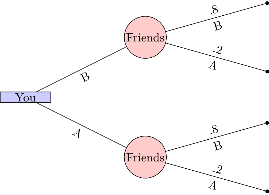
$A simple decision tree\label{L01-img01}$

The tree shows that if you were to choose your location first it would be in your interest of choosing coffee house B. This gives you an 80% chance of being in the same location as your friends.

In general these sorts of decisions are not at the mercy of chance. You would probably choose to go to coffee house A or B and simply let your friends know where you are so that they could make an informed decision. This consecutive making of decisions is a type of game.

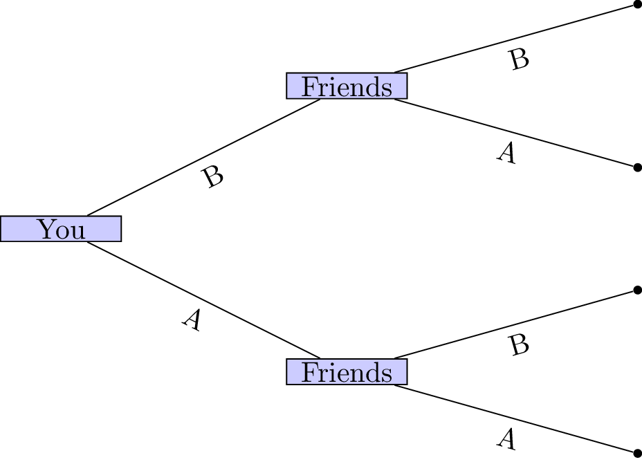
$Consecutive decisions\label{L01-img02}$

In this game the outcome (whether or not your friends and you have a coffee together) depends on the actions of all the players.

2/3rds of the average game

Let us consider another type of game:

Every player must write a whole number between 0 and 100 on the provided sheet.
The winner of the game will be the player whose number is closest to 2/3rd of the average of all the numbers written by all the players.

Extensive Form Games

We will now return to the tree diagrams drawn previously. In game theory trees are used to represent a type of game called: extensive form games.

Definition of an Extensive form game

An $N$ player extensive form game of complete information consists of:

A finite set of $N$ players;
A rooted tree (which we refer to as the game tree);
Each leaf of the tree has an $N$-tuple of payoffs;

Example: Battle of the sexes

Let’s consider the following game.

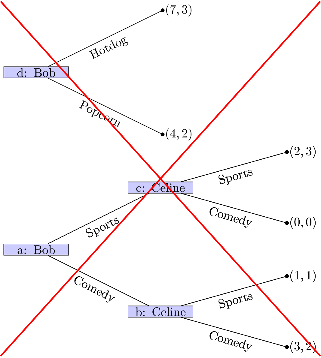
Two friends must decide what movie to watch at the cinema. Bob would like to watch a comedy and Celine would like to watch a sports movie. Importantly they would both rather spend their evening together then apart.

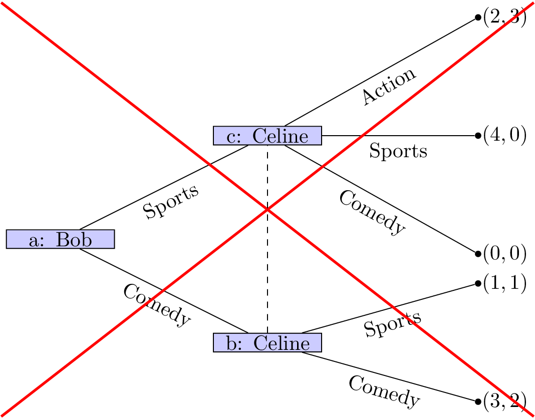
The game as well as the utilities of Bob and Celine:

$Bob and Celine\label{L01-img03}$

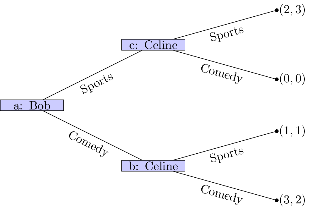
If we assume that this is the order with which decisions take place it should be relatively straightforward to predict what will happen:

Bob sees that no matter what he picks Celine will pick the same type of movie;
Bob can thus pick a comedy to ensure that he gets a slightly higher utility.

(This is actually using a process called backward induction but we’ll see that formally a bit later.)

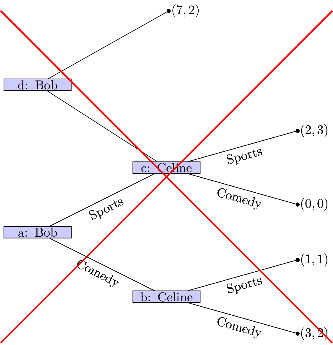
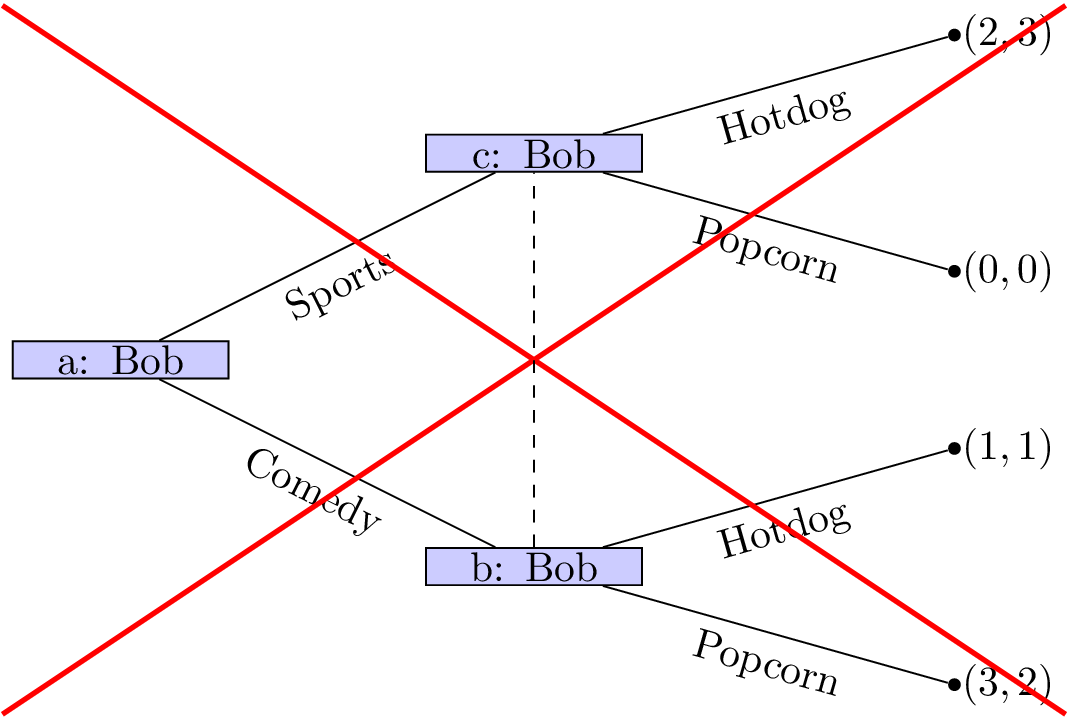
Of course we can simply represent this game in a different way (remember that in the above description we did not mention who would be making the initial decision).

$Celine and Bob\label{L01-img04}$

In this case it should again be relatively straightforward to predict what will happen:

Celine sees that no matter what she picks Bob will pick the same type of movie;
Celine can thus pick sports to ensure that she gets a slightly higher utility.

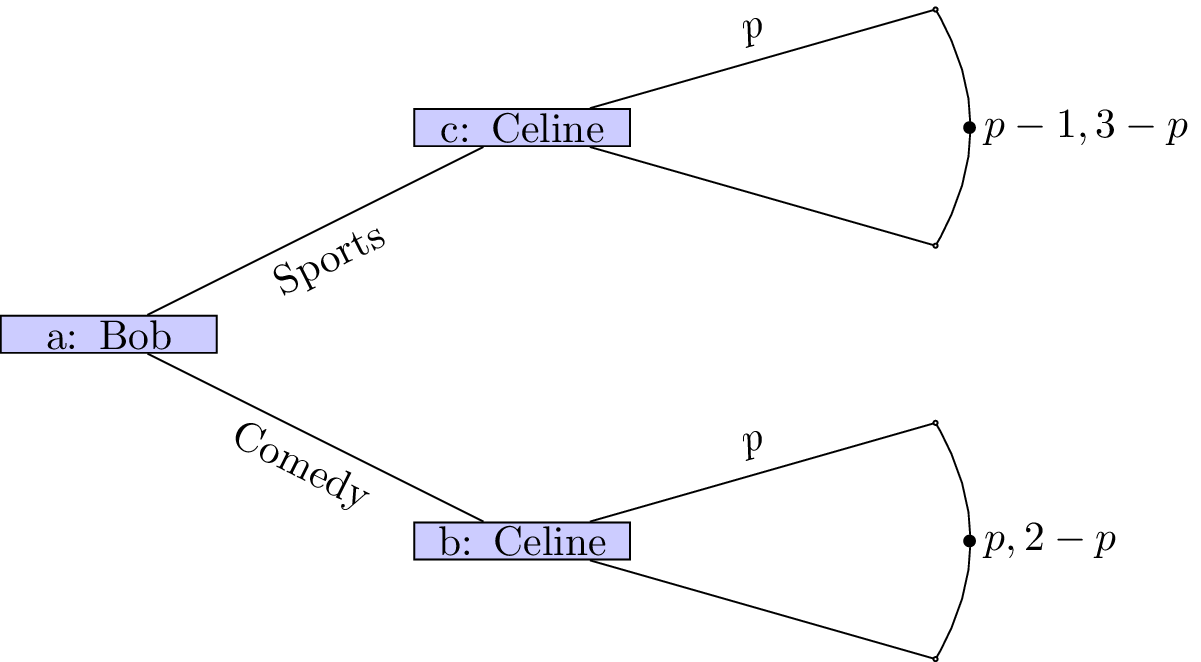
The main assumption we are making here is concerned with the amount of information available to both players at different points of the game. In both cases we have here assumed that the information available at nodes b and c is different. This is not always the case.

Information sets

Definition of an Information set

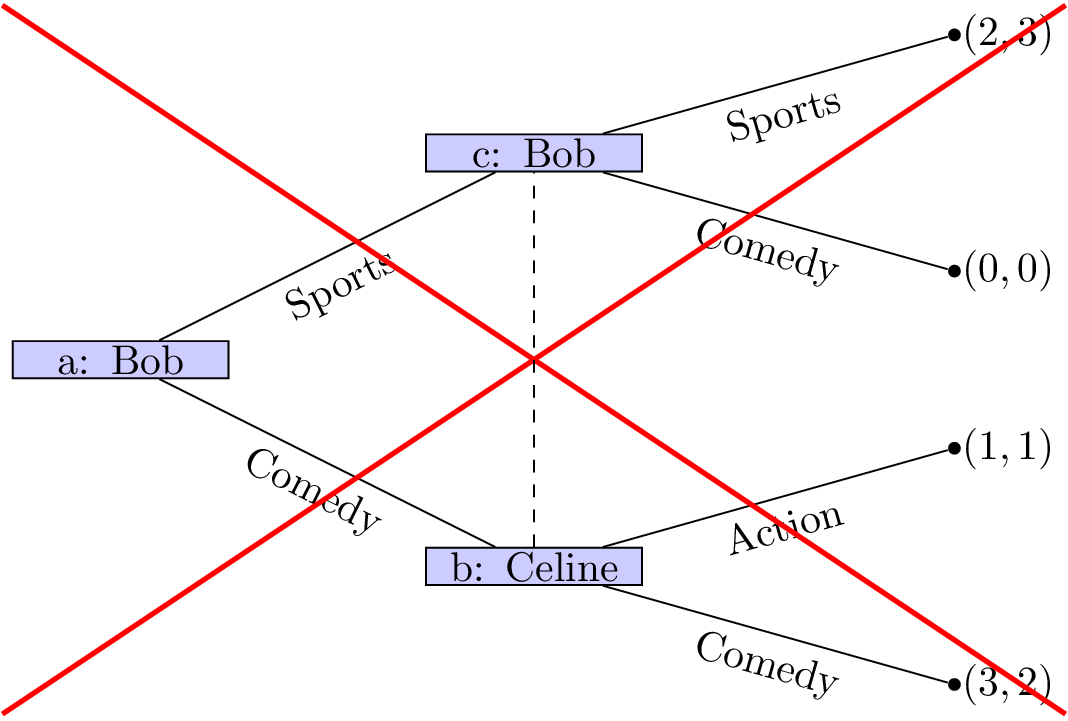
Two nodes of a game tree are said to be part of the same information set if the player at that node cannot differentiate between them.

We represent nodes being part of the same information set using a dashed line. In our example with Celine and Bob if both players must decide on a movie without knowing what the other will do we see that nodes b and c now have the same information set.

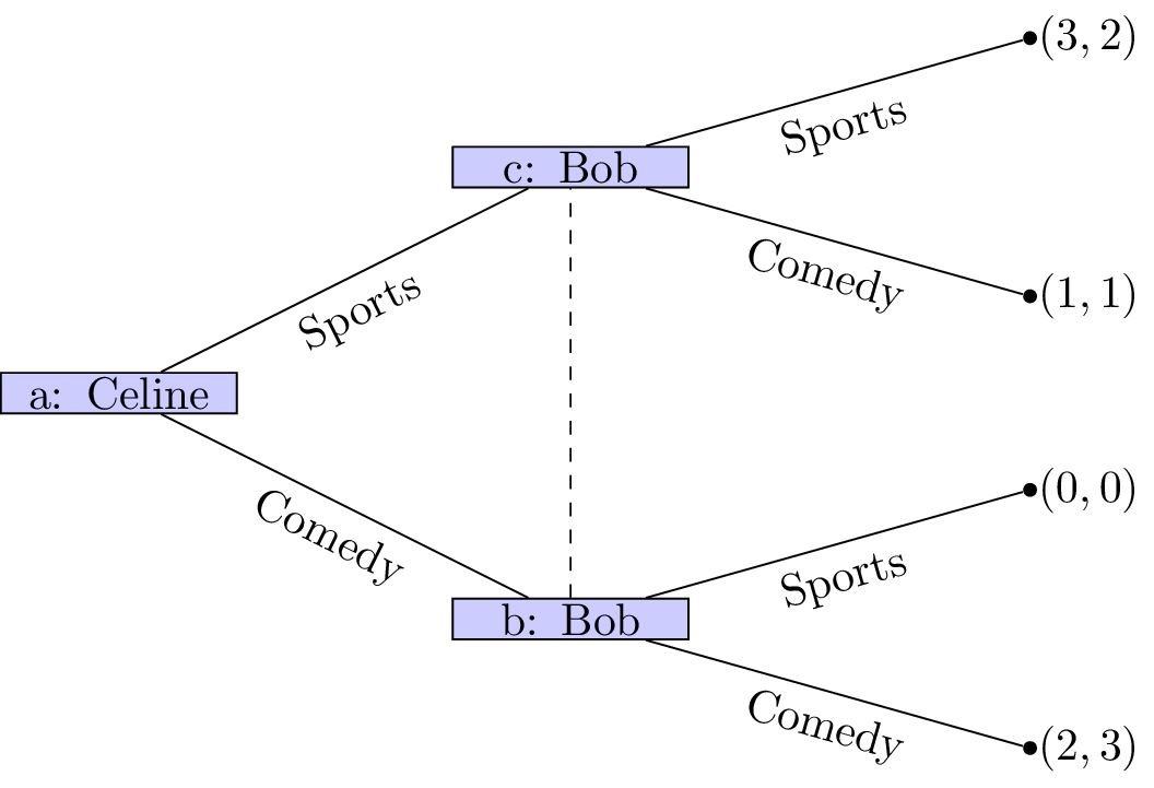
$Celine and Bob with Information Set\label{L01-img05}$

It is now a lot more difficult to try and predict the outcome of this situation.

Chapter 2 - Normal Form Games

Recap

In the previous chapter we discussed:

Interactive decision making;
Extensive form games;
Extensive form games and representing information sets.

We did this looking at a game called “the battle of the sexes”:

Celine and Bob with Information Set.

Can we think of a better way of representing this game?

Normal form games

Another representation for a game is called the normal form.

Definition of a normal form game

A $N$ player normal form game consists of:

A finite set of $N$ players;
Strategy spaces for the players: $S_1, S_2, S_3, \dots S_N$;
Payoff functions for the players: $u_i:S_{1}\times S_2\dots\times S_N\to \mathbb{R}$

The convention used in this course (unless otherwise stated) is that all players aim to choose from their strategies in such a way as to maximise their utilities.

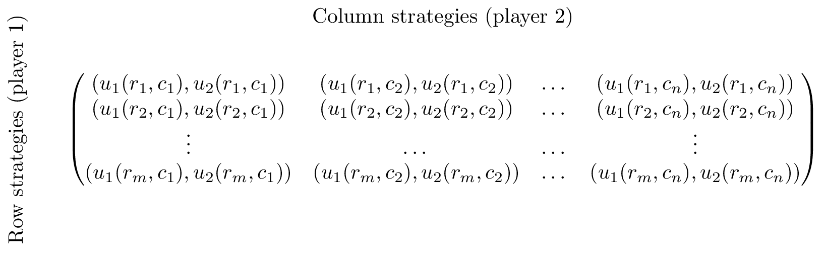
A natural way of representing a two player normal form game is using a bi-matrix. If we assume that $N=2$ and $S_1=\{r_i\;|\;1\leq i\leq m \}$ and $S_2=\{c_j\;|\;1\leq j\leq n \}$ then a bi-matrix representation of the game considered is shown.

$A bi matrix for $N=2$. \label{L02-img01}$

Some examples

The battle of the sexes

This is the game we’ve been looking at between Bob and Celine:

$\begin{pmatrix} (3,2)&(0,0)\\ (1,1)&(2,3) \end{pmatrix}$

Prisoners’ Dilemma

Assume two thieves have been caught by the police and separated for questioning. If both thieves cooperate and don’t divulge any information they will each get a short sentence. If one defects he/she is offered a deal while the other thief will get a long sentence. If they both defect they both get a medium length sentence.

$\begin{pmatrix} (2,2)&(0,3)\\ (3,0)&(1,1) \end{pmatrix}$

Hawk-Dove

Suppose two birds of prey must share a limited resource. The birds can act like a hawk or a dove. Hawks always fight over the resource to the point of exterminating a fellow hawk and/or take a majority of the resource from a dove. Two doves can share the resource.

$\begin{pmatrix} (0,0)&(3,1)\\ (1,3)&(2,2) \end{pmatrix}$

Pigs

Consider two pigs. One dominant pig and one subservient pig. These pigs share a pen. There is a lever in the pen that delivers food but if either pig pushes the lever it will take them a little while to get to the food. If the dominant pig pushes the lever, the subservient pig has some time to eat most of the food before being pushed out of the way. If the subservient pig push the lever, the dominant pig will eat all the food. Finally if both pigs go to push the lever the subservient pig will be able to eat a third of the food.

$\begin{pmatrix} (4,2)&(2,3)\\ (6,-1)&(0,0) \end{pmatrix}$

Matching pennies

Consider two players who can choose to display a coin either Heads facing up or Tails facing up. If both players show the same face then player 1 wins, if not then player 2 wins.

$\begin{pmatrix} (1,-1)&(-1,1)\\ (-1,1)&(1,-1) \end{pmatrix}$

Mixed Strategies

So far we have only considered so called pure strategies. We will now allow players to play mixed strategies.

Definition of a mixed strategy

In an $N$ player normal form game a mixed strategy for player $i$ denoted by $\sigma_i\in[0,1]^{|S_i|}_{\mathbb{R}}$ is a probability distribution over the pure strategies of player $i$. So:

$\sum_{j=1}^{|S_i|}(\sigma_i)_j=1$

For a given player $i$ we denote the set of mixed strategies as $\Delta S_i$.

For example in the matching pennies game discussed previously. A strategy profile of $\sigma_1=(.2,.8)$ and $\sigma_2=(.6,.4)$ implies that player 1 plays heads with probability .2 and player 2 plays heads with probability .6.

We can extend the utility function which maps from the set of pure strategies to $\mathbb{R}$ using expected payoffs. For a two player game we have:

$u_{i}(\sigma_1,\sigma_2)=\sum_{r\in S_1,c\in S_2}\sigma_1(r)\sigma_2(c)u_{i}(r,c)$

(where we relax our notation to allow $\sigma_i:S_i\to[0,1]_{\mathbb{R}}$ so that $\sigma_i(s_i)$ denotes the probability of playing $s_i\in S_i$.)

Matching pennies revisited.

In the previously discussed strategy profile of $\sigma_1=(.2,.8)$ and $\sigma_2=(.6,.4)$ the expected utilities can be calculated as follows:

$u_{1}(\sigma_1,\sigma_2)=\sum_{r\in S_1,c\in S_2}\sigma_1(r)\sigma_2(s)u_{1}(r,c)=.2\times.6\times 1+.2\times.4\times (-1)+.8\times .6\times (-1) + .8\times .4\times 1=-.12$ $u_{2}(\sigma_1,\sigma_2)=\sum_{r\in S_1,c\in S_2}\sigma_1(r)\sigma_2(s)u_{2}(r,c)=.2\times.6\times (-1)+.2\times.4\times 1+.8\times .6\times 1 + .8\times .4\times (-1)=.12$

Example

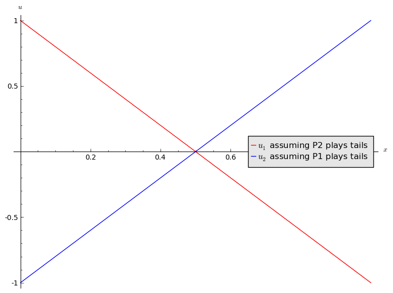
If we assume that player 2 always plays tails, what is the expected utility to player 1?

Let $\sigma_1=(x,1-x)$ and we have $\sigma_2=(0,1)$ which gives:

$u_{1}(\sigma_1,\sigma_2)=\sum_{r\in S_1,c\in S_2}\sigma_1(r)\sigma_2(c)u_{1}(r,c)=-x+(1-x)=1-2x$

Similarly if player 1 always plays tails the expected utility to player 2 is:

$u_{2}(\sigma_1,\sigma_2)=\sum_{r\in S_1,c\in S_2}\sigma_1(r)\sigma_2(c)u_{2}(r,c)=x+(x-1)=2x-1$

A plot of this is shown.

$Plot of utility if both players play tails. \label{L02-plot01}$

Add to this plot by assuming that the players independently both play heads.

Chapter 3 - Dominance

Recap

In the previous chapter we discussed:

Normal form games;
Mixed strategies and expected utilities.

We spent some time talking about predicting rational behaviour in the above games but we will now look a particular tool in a formal way.

Dominant strategies

In certain games it is evident that certain strategies should never be used by a rational player. To formalise this we need a couple of definitions.

Definition of an incomplete strategy profile

In an $N$ player normal form game when considering player $i$ we denotes by $s_{-i}$ an incomplete strategy profile for all other players in the game.

For example in a 3 player game where $S_i=\{A,B\}$ for all $i$ a valid strategy profile is $s=(A,A,B)$ while $s_{-2}=(A,B)$ denotes the incomplete strategy profile where player 1 and 3 are playing A and B (respectively).

This notation now allows us to define an important notion in game theory.

Definition of a strictly dominated strategy

In an $N$ player normal form game. A pure strategy $s_i\in S_i$ is said to be strictly dominated if there is a strategy $\sigma_i\in \Delta S_i$ such that $u_i(\sigma_i,s_{-i})>u_{i}(s_i, s_{-i})$ for all $s_{-i}\in S_{-i}$ of the other players.

When attempting to predict rational behaviour we can elimate dominated strategies.

$\begin{pmatrix} (0,1)&(3,5)\\ (5,10)&(-1,34) \end{pmatrix}$

If we let $S_1={r_1, r_2}$ and $S_2={c_1, c_2}$ we see that:

$u_2(c_2,r_1)>u_2(c_1,r_1)$ and $u_2(c_2,r_2)>u_2(c_1,r_2)$

so $c_1$ is a strictly dominated strategy for player 2. As such we can eliminate it from the game when attempting to predict rational behaviour. This gives the following game:

$\begin{pmatrix} (3,5)\\ (-1,34) \end{pmatrix}$

At this point it is straightforward to see that $r_2$ is a strictly dominated strategy for player 1 giving the following predicted strategy profile: $s=(r_1,c_2)$.

Definition of a weakly dominated strategy

In an $N$ player normal form game. A pure strategy $s_i\in S_i$ is said to be weakly dominated if there is a strategy $\sigma_i\in \Delta S_i$ such that $u_i(\sigma_i,s_{-i})\geq u_{i}(s_i,s_{-i})$ for all $s_{-i}\in S_{-i}$ of the other players and there exists a strategy profile $\bar s\in S_{-i}$ such that $u_i(\sigma_i,\bar s)> u_{i}(s_i,\bar s)$ .

We can once again predict rational behaviour by eliminating weakly dominated strategies.

As an example consider the following two player game:

$\begin{pmatrix} (3,3)&(2,2)\\ (2,1)&(2,1) \end{pmatrix}$

Using the same convention as before for player 2, $c_1$ weakly dominates $c_2$ and for player 1, $r_1$ weakly dominates $r_2$ giving the following predicted strategy profile $(r_1,c_1)$.

Common knowledge of rationality

An important aspect of game theory and the tool that we have in fact been using so far is to assume that players are rational. However we can (and need) to go further:

The players are rational;
The players all know that the other players are rational;
The players all know that the other players know that they are rationals;
…

This chain of assumptions is called Common knowledge of rationality (CKR). By applying the CKR assumption we can attempt to predict rational behaviour through the iterated elimination of dominated strategies (as we have been doing above).

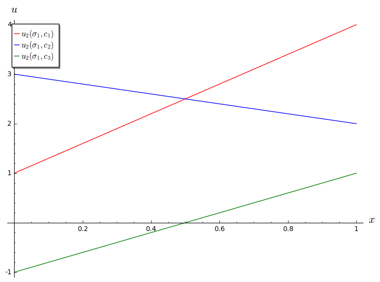
Example

Let us try to predict rational behaviour in the following game using iterated elimination of dominated strategies:

$\begin{pmatrix} (1,0)&(1,2)&(0,1)\\ (0,3)&(0,1)&(2,0) \end{pmatrix}$

Initially player 1 has no dominated strategies. For player 2, $c_3$ is dominated by $c_2$. Now $r_2$ is dominated by $r_1$ for player 1. Finally, $c_1$ is dominated by $c_2$. Thus $(r_1,c_2)$ is a predicted rational outcome.

Example

Let us try to predict rational behaviour in the following game using iterated elimination of dominated strategies:

$\begin{pmatrix} (10,1)&(5,1)&(1,-2)\\ (10,1)&(5,0)&(4,2) \end{pmatrix}$

$r_1$ weakly dominated by $r_2$
$c_1$ strictly dominated by $c_3$
$c_2$ strictly dominated by $c_1$

Thus $(r_2,c_3)$ is a predicted rational outcome.

Not all games can be solved using dominance

Consider the following two games:

$\begin{pmatrix} (3,2)&(0,0)\\ (1,1)&(2,3) \end{pmatrix}$ $\begin{pmatrix} (1,3)&(4,2)&(2,2)\\ (4,0)&(0,3)&(4,1)\\ (2,5)&(3,4)&(5,6) \end{pmatrix}$

Why can’t we predict rational behaviour using dominance?

Chapter 4 - Best responses

Recap

In the previous chapter we discussed:

Predicting rational behaviour using dominated strategies;
The CKR;

We did discover certain games that did not have any dominated strategies.

Best response functions

Definition of a best response

In an $N$ player normal form game. A strategy $s^*$ for player $i$ is a best response to some strategy profile $s_{-i}$ if and only if $u_i(s^*,s_{-i})\geq u_{i}(s,s_{-i})$ for all $s\in S_i$.

We can now start to predict rational outcomes in pure strategies by identifying all best responses to a strategy.

$\begin{pmatrix} (1,3)&(4,2)&(2,2)\\ (4,0)&(0,3)&(4,1)\\ (2,5)&(3,4)&(5,6) \end{pmatrix}$

We will underline the best responses for each strategy giving ($r_i$ is underlined if it is a best response to $s_j$ and vice versa):

$\begin{pmatrix} (1,\underline{3})&(\underline{4},2)&(2,2)\\ (\underline{4},0)&(0,\underline{3})&(4,1)\\ (2,5)&(3,4)&(\underline{5},\underline{6}) \end{pmatrix}$

We see that $(r_3,c_3)$ represented a pair of best responses. What can we say about the long term behaviour of this game?

Best responses against mixed strategies

We can identify best responses against mixed strategies. Let us take a look at the matching pennies game:

$\begin{pmatrix} (1,-1)&(-1,1)\\ (-1,1)&(1,-1) \end{pmatrix}$

If we assume that player 2 plays a mixed strategy $\sigma_2=(x,1-x)$ we have:

$u_1(r_1,\sigma_2)=2x-1$

and

$u_1(r_2,\sigma_2)=1-2x$

$Mixed strategies fox the matching pennies game. \label{L04-plot01}$

We see that:

If $x<1/2$ then $r_2$ is a best response for player 1.
If $x>1/2$ then $r_1$ is a best response for player 1.
If $x=1/2$ then player 1 is indifferent.

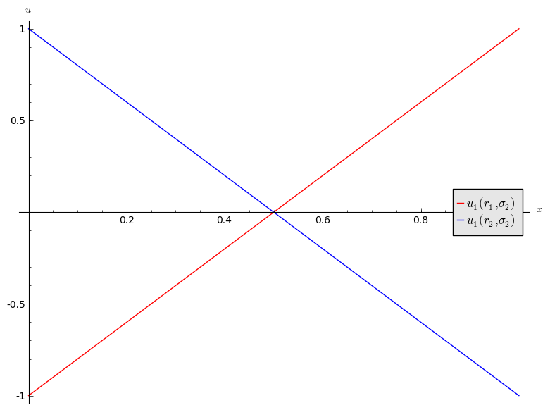
Let us repeat this exercise for the battle of the sexes game.

$\begin{pmatrix} (3,2)&(0,0)\\ (1,1)&(2,3) \end{pmatrix}$

If we assume that player 2 plays a mixed strategy $\sigma_2=(x,1-x)$ we have:

$u_1(r_1,\sigma_2)=3x$

and

$u_1(r_2,\sigma_2)=2-x$

$Mixed strategies for the battle of the sexes game. \label{L04-plot02}$

We see that:

If $x<1/2$ then $r_2$ is a best response for player 1.
If $x>1/2$ then $r_1$ is a best response for player 1.
If $x=1/2$ then player 1 is indifferent.

Connection between best responses and dominance

Definition of the undominated strategy set

In an $N$ player normal form game, let us define the undominated strategy set $UD_i$:

$UD_i=\{s\in S_i\;|\; \text{s is not strictly dominated}\}$

If we consider the following game:

$\begin{pmatrix} (3,3)&(7,2)&(5,1)\\ (5,1)&(6,3)&(7,-1) \end{pmatrix}$

We have:

$UD_1=\{r_1,r_2\}$ $UD_2=\{c_1,c_2\}$

Definition of the best responses strategy set

In an $N$ player normal form game, let us define the best responses strategy set $B_i$:

$B_i=\{s\in S_i\;|\; \exists\;\sigma\in\Delta S_{-i}\text{ such that }s \text{ is a best response to }\sigma\}$

In other words $B_i$ is the set of functions that are best responses to some strategy profile in $S_{-i}$.

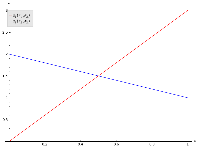
Let us try to identify $B_2$ for the above game. Let us assume that player 1 plays $\sigma_1=(x,1-x)$. This gives:

$u_2(\sigma_1,c_1)=1+2x$ $u_2(\sigma_1,c_2)=3-x$ $u_2(\sigma_1,c_3)=2x-1$

Plotted:

$Utilities of player 2 in our example. \label{L04-plot03}$

We see that $c_3$ is never a best response for player 2:

$B_2=\{c_1,c_2\}$

We will now attempt to identify $B_1$ for the above game. Let us assume that player two plays $\sigma_2=(x,y,1-x-y)$. This gives:

$u_1(r_1,\sigma_2)=xu_1(r_1,c_1)+yu_1(r_1,c_2)+(1-x-y)u_1(r_1,c_3)=3x+7y+5-5y-5x$ $u_1(r_2,\sigma_2)=xu_1(r_2,c_1)+yu_1(r_2,c_2)+(1-x-y)u_1(r_2,c_3)=5x+6y+7-7y-7x$

$u_1(r_1,\sigma_2)-u_1(r_2,\sigma_2)=3y - 2$

If we can find values of $y$ that give valid $\sigma_2=(x,y,1-x-y)$ and that make the above difference both positive and negative then:

$B_1=\{r_1,r_2\}$

$y=1$ gives $u_1(r_1,\sigma_2)-u_2(r_2,\sigma_2)=1>0$ (thus $r_1$ is best response to $\sigma_2=(0,1,0)$). Similarly, $y=0$ gives $u_1(r_1,\sigma_2)-u_2(r_2,\sigma_2)=-2<0$ (thus $r_2$ is best response to $\sigma_2=(x,0,1-x)$ for any $0\leq x \leq 1$) as required.

We have seen in our example that $B_i=UD_i$. This leads us to two Theorems (the proofs are omitted).

Theorem of equality in 2 player games

In a 2 player normal form game $B_i=UD_i$ for all $i\in{1,2}$.

This is however not always the case:

Theorem of inclusion in $N$ player games

In an $N$ player normal form game $B_i\subseteq UD_i$ for all $1 \leq i\leq n$.

Chapter 5 - Nash equilibria in pure strategies

Recap

In the previous chapter we discussed:

The definition of best responses;
The connection between dominance and best responses;
Best responses against mixed strategies.

So far we have been using various tools to loosely discuss ‘predicting rational behaviour’. We will now formalise what we mean.

Nash equilibria

Definition of Nash equilibria

In an $N$ player normal form game. A Nash equilibrium is a strategy profile $\tilde s = (\tilde s_1,\tilde s_2,\dots,\tilde s_N)$ such that:

$u_i(\tilde s)\geq u_i(\bar s_i,\tilde s_{-i})\text{ for all }i$

This implies that all strategies in the strategy profile $\tau$ are best responses to all the other strategies.

An important interpretation of this definition is that at the Nash equilibria no player has an incentive to deviate from their current strategy.

To find Nash equilibria in 2 player normal form games we can simply check every strategy pair and see whether or not a player has an incentive to deviate.

Example

Identify Nash equilibria in pure strategies for the following game:

$\begin{pmatrix} (0,3)&(1,2)&(7,8)&(1,4)\\ (2,6)&(1,2)&(3,0)&(1,3)\\ (3,1)&(1,2)&(3,-1)&(5,1)\\ (6,3)&(4,2)&(2,1)&(7,1) \end{pmatrix}$

If we identify all best responses:

$\begin{pmatrix} (0,3)&(1,2)&(\underline{7},\underline{8})&(1,4)\\ (2,\underline{6})&(1,2)&(3,0)&(1,3)\\ (3,1)&(1,\underline{2})&(3,-1)&(5,1)\\ (\underline{6},\underline{3})&(\underline{4},2)&(2,1)&(\underline{7},1) \end{pmatrix}$

We see that we have 2 equilibria in pure strategies: $(r_1,c_3)$ and $(r_4,c_1)$

Duopoly game

We will now consider a particular normal form game attributed to Augustin Cournot.

Suppose that two firms 1 and 2 produce an identical good (ie consumers do not care who makes the good). The firms decide at the same time to produce a certain quantity of goods: $q_1,q_2\geq 0$. All of the good is sold but the price depends on the number of goods:

$p=K-q_1-q_2$

We also assume that the firms both pay a production cost of $k$ per goods.

What is the Nash equilibria for this game?

Firstly let us clarify that this is indeed a normal form game:

2 players;
The strategy space is $S_1=S_2=\mathbb{R}_{\geq 0}$
The utilities are given by:

$u_1(q_1,q_2)=(K-q_1-q_2)q_1-kq_1$ $u_2(q_1,q_2)=(K-q_1-q_2)q_2-kq_2$

Let us now compute the best responses for each firm (we’ll in fact only need to do this for one firm given the symmetry of the problem).

$\frac{du_1}{dq_1}=K-2q_1-q_2-k$

Setting this to 0 gives the best response $q_1^*=q_1^*(q_2)$ for firm 1:

$q_1^*(q_2)=\frac{K-k-q_2}{2}$

By symmetry we have:

$q_2^*(q_1)=\frac{K-k-q_1}{2}$

Recalling the definition of a Nash equilibria we are attempting to find $(\tilde q_1, \tilde q_2)$ a pair of best responses. Thus $\tilde q_1$ satisfies:

$\begin{cases} \tilde q_1=q_1^*(\tilde q_2)\\ \tilde q_2=q_2^*(\tilde q_1) \end{cases}$ $\Leftrightarrow$ $\begin{cases} \tilde q_1=\frac{K-k-\tilde q_2}{2}\\ \tilde q_2=\frac{K-k-\tilde q_1}{2} \end{cases}$ $\Leftrightarrow$ $\begin{cases} \tilde q_1=\frac{K-k}{3}\\ \tilde q_2=\frac{K-k}{3}\\ \end{cases}$

Chapter 6 - Nash equilibria in mixed strategies

Recap

In the previous chapter

The definition of Nash equilibria;
Identifying Nash equilibria in pure strategies;
Solving the duopoly game;

This brings us to a very important part of the course. We will now consider equilibria in mixed strategies.

Recall of expected utility calculation

In the matching pennies game discussed previously:

$\begin{pmatrix} (1,-1)&(-1,1)\\ (-1,1)&(1,-1) \end{pmatrix}$

Recalling Chapter 2 a strategy profile of $\sigma_1=(.2,.8)$ and $\sigma_2=(.6,.4)$ implies that player 1 plays heads with probability .2 and player 2 plays heads with probability .6.

We can extend the utility function which maps from the set of pure strategies to $\mathbb{R}$ using expected payoffs. For a two player game we have:

$u_{i}(\sigma_1,\sigma_2)=\sum_{r\in S_1,c\in S_2}\sigma_1(r)\sigma_2(c)u_{i}(r,c)$

Obtaining equilibria

Let us investigate the best response functions for the matching pennies game.

If we assume that player 2 plays a mixed strategy $\sigma_2=(y,1-y)$ we have:

$u_1(r_1,\sigma_2)=2y-1$ and $u_1(r_2,\sigma_2)=1-2y$

shown:

$Utilities of player 1 in the matching pennies game.\label{L06-plot01}$

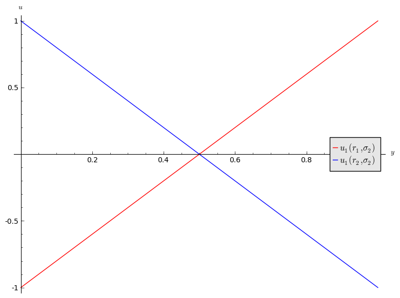
If $y<1/2$ then $r_2$ is a best response for player 1.
If $y>1/2$ then $r_1$ is a best response for player 1.
If $y=1/2$ then player 1 is indifferent.

If we assume that player 1 plays a mixed strategy $\sigma_1=(x,1-x)$ we have:

$u_2(\sigma_1,c_1)=1-2x$ and $u_2(\sigma_1,c_2)=2x-1$

shown:

$Utilities of player 2 in the matching pennies game.\label{L06-plot02}$

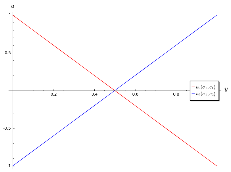
Thus we have:

If $x<1/2$ then $c_1$ is a best response for player 2.
If $x>1/2$ then $c_2$ is a best response for player 2.
If $x=1/2$ then player 2 is indifferent.

Let us draw both best responses on a single diagram, indicating the best responses in each quadrant. The arrows show the deviation indicated by the best responses.

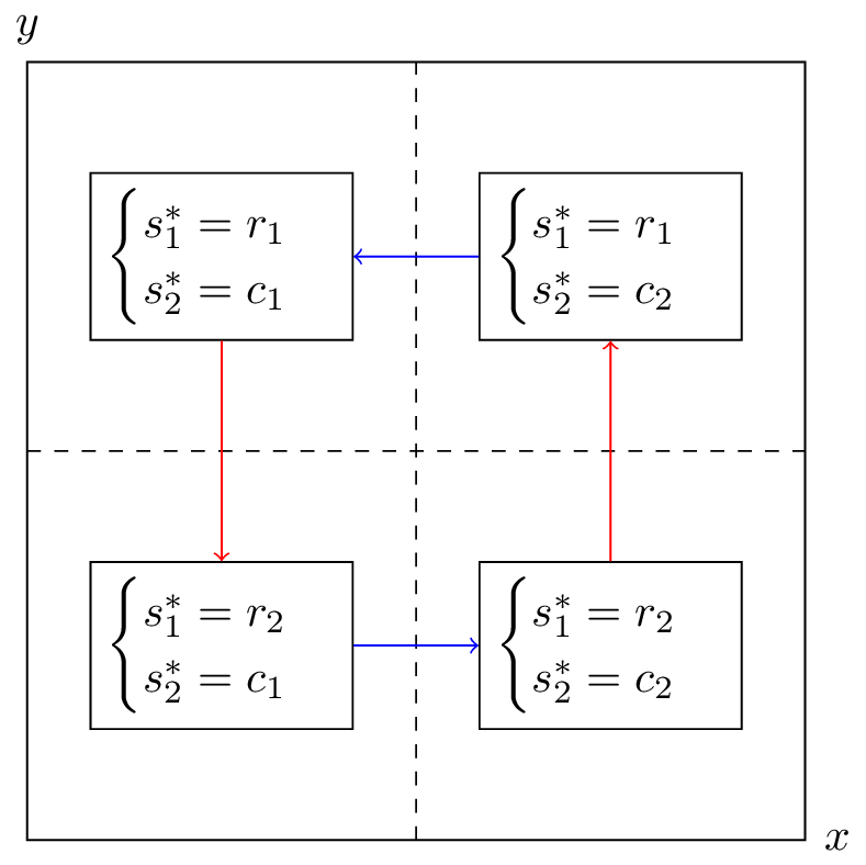
$Best response moves based on current strategy. \label{L06-img01}$

If either player plays a mixed strategy other than $(1/2,1/2)$ then the other player has an incentive to modify their strategy. Thus the Nash equilibria is:

$((1/2,1/2),(1/2,1/2))$

This notion of “indifference” is important and we will now prove an important theorem that will prove useful when calculating Nash Equilibria.

Equality of payoffs theorem

Definition of the support of a strategy

In an $N$ player normal form game the support of a strategy $\sigma\in\Delta S_i$ is defined as: $\mathcal{S}(\sigma)=\{s\in S_i\;|\;\sigma(s)>0\}$

I.e. the support of a strategy is the set of pure strategies that are played with non zero probability.

For example, if the strategy set is ${A,B,C}$ and $\sigma=(1/3,2/3,0)$ then $\mathcal{S}(\sigma)={A,B}$.

Theorem of equality of payoffs

In an $N$ player normal form game if the strategy profile $(\sigma_i,s_{-i})$ is a Nash equilibria then:

$u_{i}(\sigma_i,s_{-i})=u_{i}(s,s_{-i})\text{ for all }s\in\mathcal{S}(\sigma_i)\text{ for all }1\leq i\leq N$

Proof

If $|\mathcal{S}(\sigma_i)|=1$ then the proof is trivial.

We assume that $|\mathcal{S}(\sigma_i)|>1$. Let us assume that the theorem is not true so that there exists $\bar s\in\mathcal{S}(\sigma)$ such that

$u_{i}(\sigma_i,s_{-i})\ne u_{i}(\bar s,s_{-i})$

Without loss of generality let us assume that:

$\bar s=\text{argmax}_{s\in\mathcal{S}(\sigma)}u_i(s,s_{-i})$

Thus we have:

$\begin{aligned} u_i(\sigma_i,s_{-i})&=\sum_{s\in\mathcal{S}(\sigma_i)}\sigma_i(s)u(s,s_{-i})\\ &\leq \sum_{s\in\mathcal{S}(\sigma_i)}\sigma_i(s)u(\bar s,s_{-i})\\ &\leq u(\bar s,s_{-i})\sum_{s\in\mathcal{S}(\sigma_i)}\sigma_i(s)\\ &\leq u(\bar s,s_{-i})\\ \end{aligned}$

Giving:

$u_{i}(\sigma_i,s_{-i})< u_{i}(\bar s,s_{-i})$

which implies that $(\sigma_i,s_{-i})$ is not a Nash equilibrium.

Example

Let’s consider the matching pennies game yet again. To use the equality of payoffs theorem we identify the various supports we need to try out. As this is a $2\times 2$ game we can take $\sigma_1=(x,1-x)$ and $\sigma_2=(y,1-y)$ and assume that $(\sigma_1,\sigma_2)$ is a Nash equilibrium.

from the theorem we have that $u_1(\sigma_1,\sigma_2)=u_1(r_1,\sigma_2)=u_1(r_2,\sigma_2)$

$\begin{aligned} u_1(r_1,\sigma_2)&=u_1(r_2,\sigma_2)\\ y-(1-y)&=-y+(1-y)\\ y&=1/2 \end{aligned}$

Thus we have found player 2’s Nash equilibrium strategy by finding the strategy that makes player 1 indifferent. Similarly for player 1:

$\begin{aligned} u_2(\sigma_1,c_1)&=u_2(\sigma_1,c_2)\\ -x+(1-x)&=x-(1-x)\\ x&=1/2 \end{aligned}$

Thus the Nash equilibria is:

$((1/2,1/2),(1/2,1/2))$

To finish this chapter we state a famous result in game theory:

Nash’s Theorem

Every normal form game with a finite number of pure strategies for each player, has at least one Nash equilibrium.

Chapter 7 - Extensive form games and backwards induction

Recap

In the previous chapter

We completed our look at normal form games;
Investigated using best responses to identify Nash equilibria in mixed strategies;
Proved the Equality of Payoffs theorem which allows us to compute the Nash equilibria for a game.

In this Chapter we start to look at extensive form games in more detail.

Extensive form games

If we recall Chapter 1 we have seen how to represent extensive form games as a tree.

$Bob and Celine. \label{L01-img03}$

We will now consider the properties that define an extensive form game game tree:

Every node is a successor of the (unique) initial node.

$A tree with two initial nodes.\label{L07-img01}$
Every node apart from the initial node has exactly one predecessor. The initial node has no predecessor.

$A tree with node c having multiple predecessors. \label{L07-img02}$
All edges extending from the same node have different action labels.

$Nodes with same action labels.\label{L07-img03}$
Each information set contains decision nodes for one player.

$Information sets with different action labels.\label{L07-img04}$
All nodes in a given information set must have the same number of successors (with the same action labels on the corresponding edges).

$Information set with different number of action edges. \label{L07-img05}$
We will only consider games with “perfect recall”, ie we assume that players remember their own past actions as well as other past events.

$A game without perfect recall.\label{L07-img06}$
If a player’s action is not a discrete set we can represent this as shown.

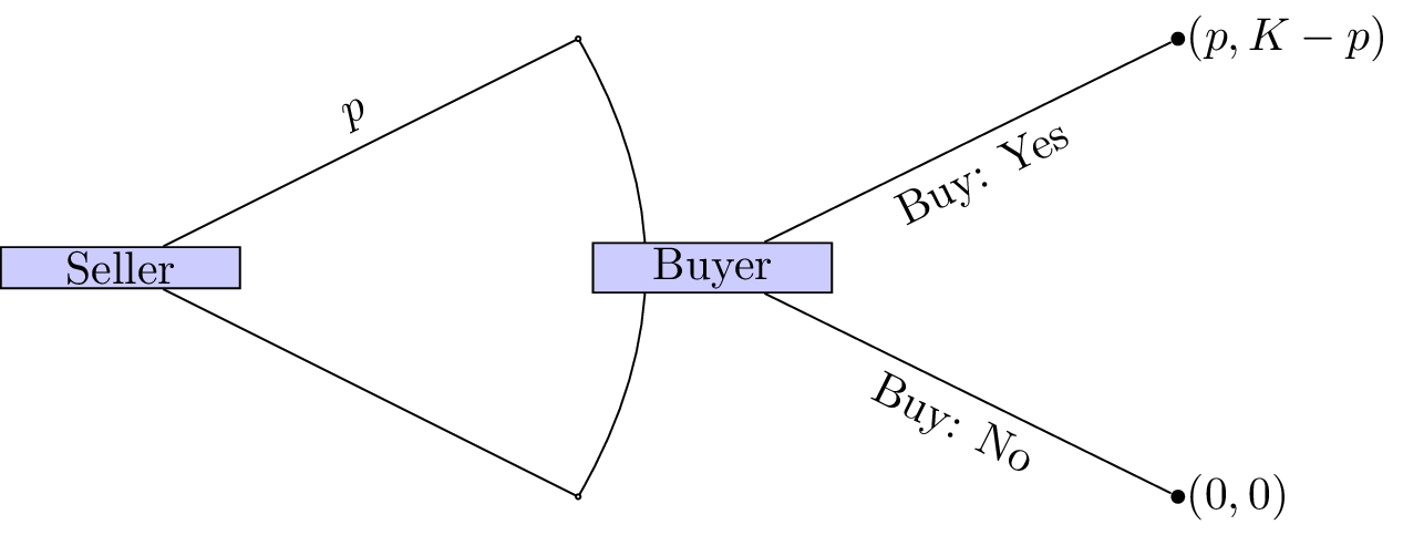
$A game tree with continuous strategy set.\label{L07-img07}$

As an example consider the following game (sometimes referred to as “ultimatum bargaining”):

Consider two individuals: a seller and a buyer. A seller can set a price $p$ for a particular object that has value $K$ to the buyer and no value to the seller. Once the sellers sets the price the buyer can choose whether or not to pay the price. If the buyer chooses to not pay the price then both players get a payoff of 0.

We can represent this.

$The seller buyer game.\label{L07-img08}$

How we can we analyse extensive form games?

Backwards induction

To analyse such games we assume that players not only attempt to optimize their overall utility but optimize their utility conditional on any information set.

Definition of sequential rationality

Sequential rationality: An optimal strategy for a player should maximise that player’s expected payoff, conditional on every information set at which that player has a decision.

With this notion in mind we can now define an analysis technique for extensive form games:

Definition of backward induction

Backward induction: This is the process of analysing a game from back to front. At each information set we remove strategies that are dominated.

Example

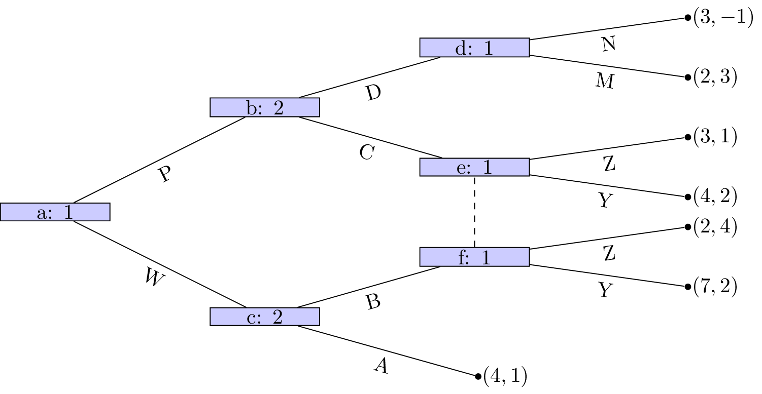
Let us consider the game shown.

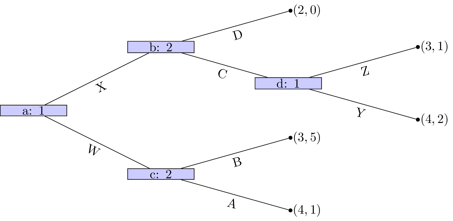
$Running example for backward induction.\label{L07-img09}$

We see that at node $(d)$ that Z is a dominated strategy. So that the game reduces to as shown.

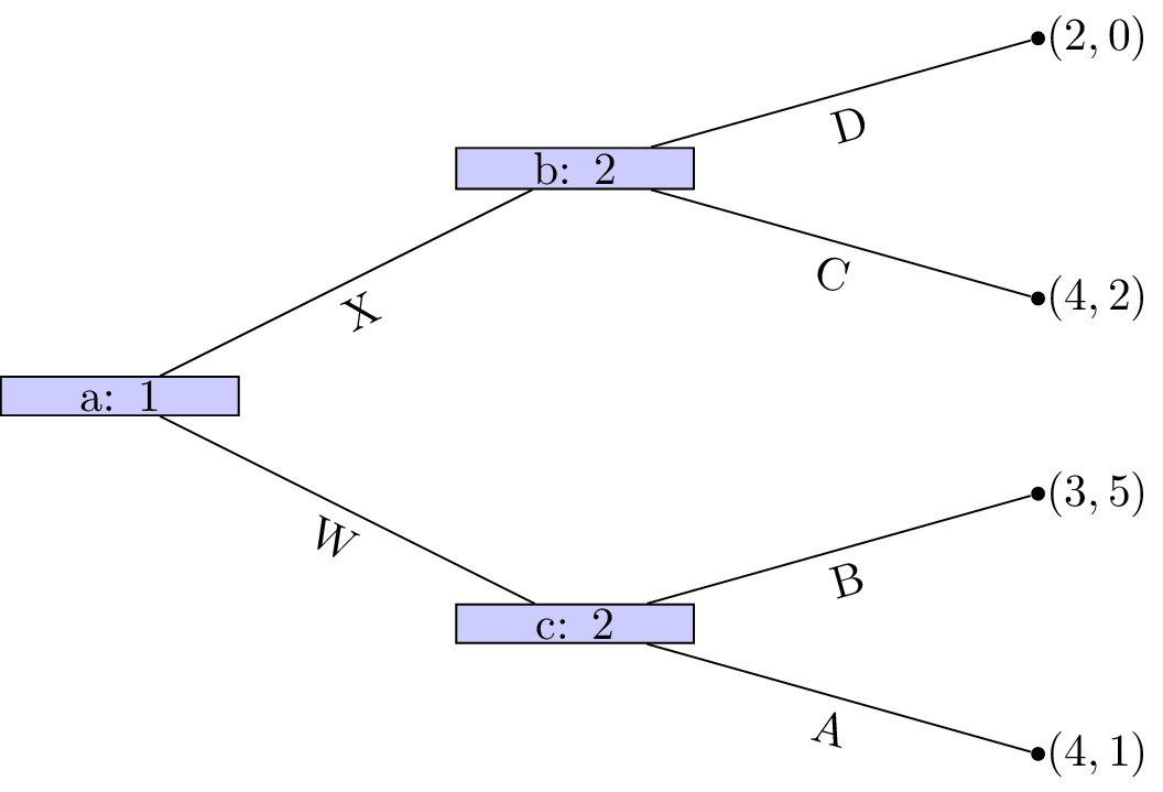
$Running example step 1.\label{L07-img10}$

Player 1s strategy profile is (Y) (we will discuss strategy profiles for extensive form games more formally in the next chapter). At node $(c)$ A is a dominated strategy so that the game reduces as shown.

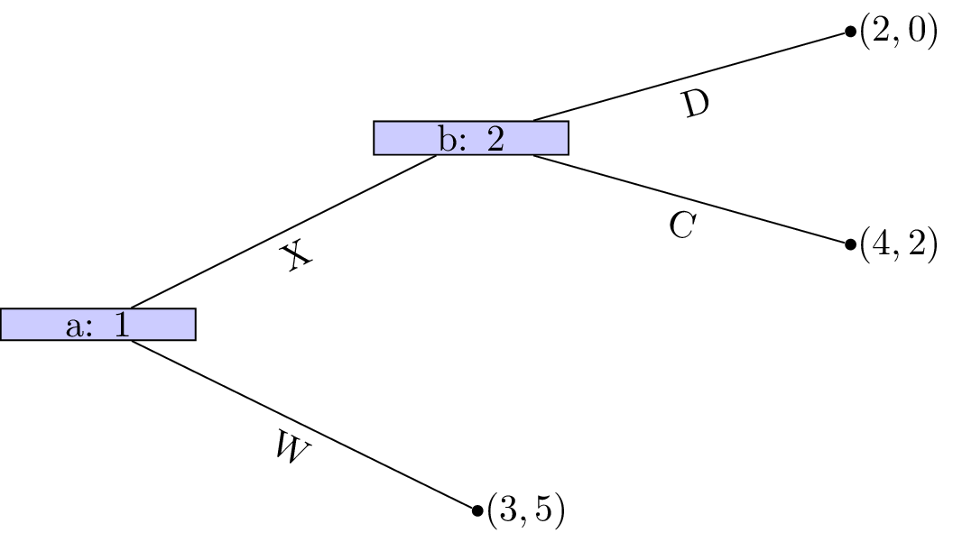
$Running example step 2.\label{L07-img11}$

Player 2s strategy profile is (B). At node $(b)$ D is a dominated strategy so that the game reduces as shown.

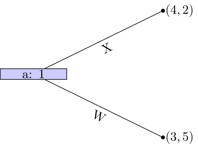
$Running example step 3.\label{L07-img12}$

Player 2s strategy profile is thus (C,B) and finally strategy W is dominated for player 1 whose strategy profile is (X,Y).

This outcome is in fact a Nash equilibria! Recalling the original tree neither player has an incentive to move.

Theorem of existence of Nash equilibrium in games of perfect information.

Every finite game with perfect information has a Nash equilibrium in pure strategies. Backward induction identifies an equilibrium.

Proof

Recalling the properties of sequential rationality we see that no player will have an incentive to deviate from the strategy profile found through backward induction. Secondly ever finite game with perfect information can be solved using backward inductions which gives the result.

Stackelberg game

Let us consider the Cournot duopoly game of Chapter 5. Recall:

Suppose that two firms 1 and 2 produce an identical good (ie consumers do not care who makes the good). The firms decide at the same time to produce a certain quantity of goods: $q_1,q_2\geq 0$. All of the good is sold but the price depends on the number of goods:

$p=K-q_1-q_2$

We also assume that the firms both pay a production cost of $k$ per bricks.

However we will modify this to assume that there is a leader and a follower, ie the firms do not decide at the same time. This game is called a Stackelberg leader follower game.

Let us represent this as a normal form game.

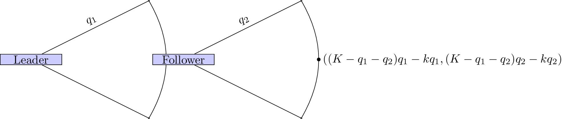
$A Stackelberg leader follower game.\label{L07-img13}$

We use backward induction to identify the Nash equilibria. The dominant strategy for the follower is:

$q_2^*(q_1)=\frac{K-k-q_1}{2}$

The game thus reduces as shown.

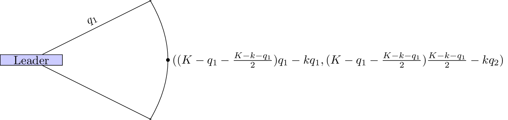
$A step of backward induction in the Stackelberg game.\label{L07-img14}$

The leader thus needs to maximise:

$u_1(q_1)=(K-q_1-\frac{K-k-q_1}{2})q_1-kq_1=(\frac{K-q_1+k}{2})q_1-kq_1$

Differentiating and equating to 0 gives:

$q_1^*=\frac{K-k}{2}$ which in turn gives: $q_2^*=\frac{K-k}{4}$

The total amount of goods produced is $\frac{3(K-k)}{4}$ whereas in the Cournot game the total amount of good produced was $\frac{2(K-k)}{3}$. Thus more goods are produced in the Stackelberg game.

Chapter 8 - Subgame Perfection

Recap

In the previous chapter

We took a formal look at extensive form games;
Investigated an analysis technique for extensive form games called backwards induction.

In this Chapter we will take a look at another important aspect of extensive form games.

Connection between extensive and normal form games

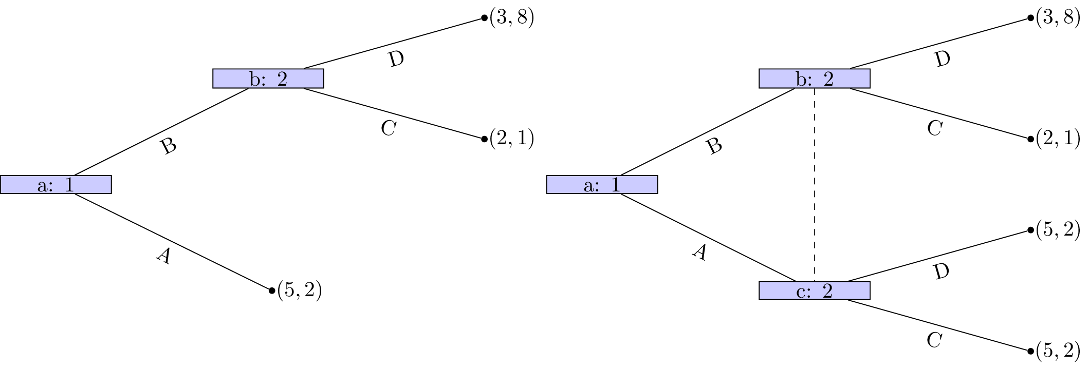
It should be relatively straightforward to see that we can represent any extensive form game in normal form. The strategies in the normal form game simply correspond to all possible combinations of strategies at each level corresponding to each player. Consider the following game:

$An extensive form game.\label{L07-img09}$

We have:

$S_1=\{\text{XY},\text{XZ},\text{WY},\text{WZ}\}$

and

$S_2=\{\text{DA},\text{DB},\text{CA},\text{CB}\}$

the corresponding normal form game is given as:

$\begin{pmatrix} (2,0)&(2,0)&(4,2)&(4,2)\\ (2,0)&(2,0)&(3,1)&(3,1)\\ (4,1)&(3,5)&(4,1)&(3,5)\\ (4,1)&(3,5)&(4,1)&(3,5) \end{pmatrix}$

Note! There is always a unique normal form representation of an extensive form game (ignoring ordering of strategies) however the opposite is not true. The following game:

$\begin{pmatrix} (3,8)&(2,1)\\ (5,2)&(5,2) \end{pmatrix}$

has the two extensive form game representations shown.

$Two extensive form games corresponding to the same extensive form game.\label{L08-img04}$

Subgames

Definition of a subgame

In an extensive form game, a node $x$ is said to initiate a subgame if and only if $x$ and all successors of $x$ are in information sets containing only successors of $x$.

A game where all nodes initiate a subgame is shown.

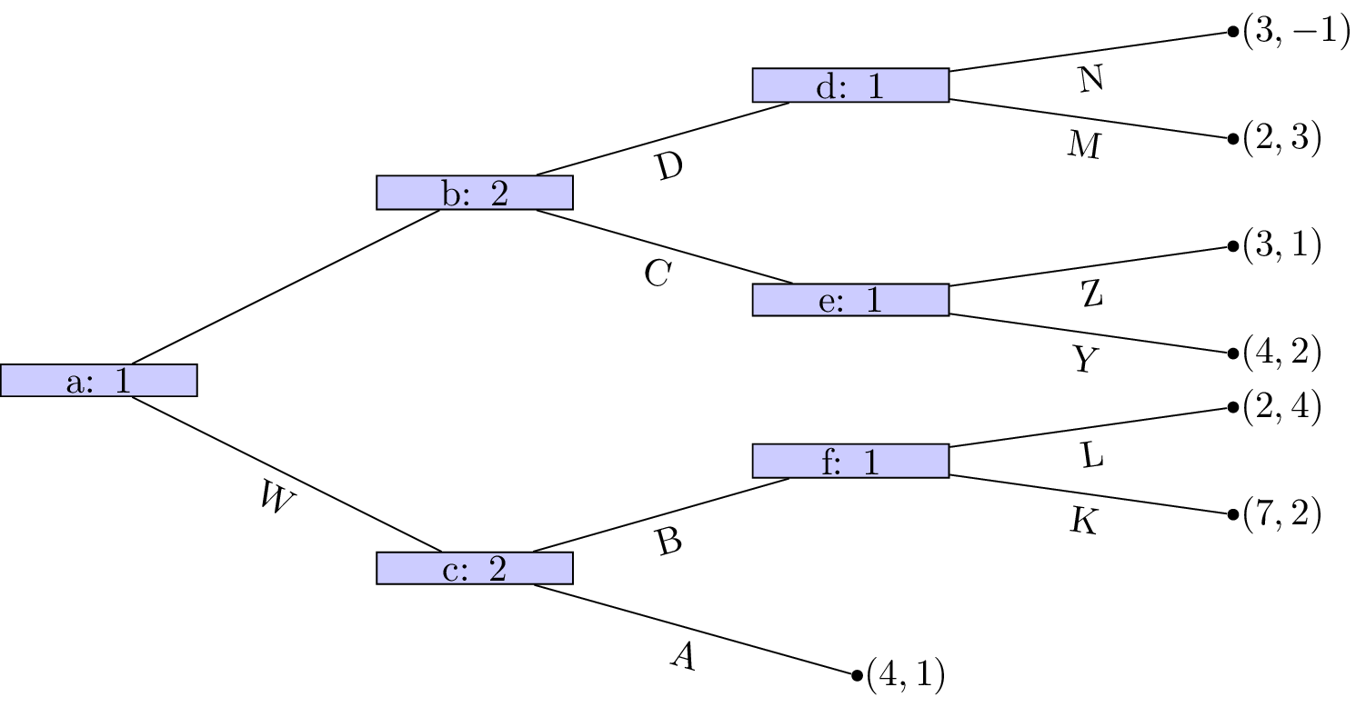
$All nodes initiate a subgame.\label{L08-img01}$

A game that does not have perfect information nodes $c$, $f$ and $b$ initiate subgames but all of $b$’s successors do not is shown.

$Nodes c,f and b initiate a subgame.\label{L08-img02}$

Similarly, in the game shown the only node that initiates a subgame is $d$.

$Node d initiates a subgame.\label{L08-img03}$

Subgame perfect equilibria

We have identified how to obtain Nash equilibria in extensive form games. We now give a refinement of this:

Definition of subgame perfect equilibrium

A subgame perfect Nash equilibrium is a Nash equilibrium in which the strategy profiles specify Nash equilibria for every subgame of the game.

Note that this includes subgames that might not be reached during play!

Let us consider the example shown.

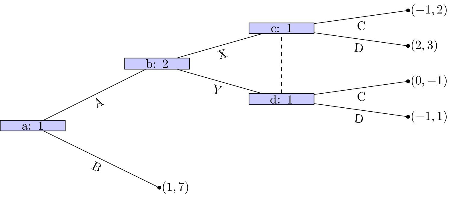
$A running example of a game with subgame perfect equilibrium.\label{L08-img05}$

Let us build the corresponding normal form game:

$S_1=\{AC,AD,BC,BD\}$ and $S_2=\{X,Y\}$

using the above ordering we have:

$\begin{pmatrix} (-1,2)&(0,-1)\\ (2,3)&(-1,1)\\ (1,7)&(1,7)\\ (1,7)&(1,7) \end{pmatrix}$

The Nash equilibria for the above game (easily found by inspecting best responses) are:

$\{(AD,X),(BC,Y),(BD,Y)\}$

If we take a look at the normal form game representation of the subgame initiated at node b with strategy sets:

$S_1=\{C,D\}\text{ and }S_2=\{X,Y\}$

we have:

$\begin{pmatrix} (-1,2)&(0,-1)\\ (2,3)&(-1,1) \end{pmatrix}$

We see that the (unique) Nash equilibria for the above game is $(D,X)$. Thus the only subgame perfect equilibria of the entire game is ${AD,X}$.

Some comments:

Hopefully it is clear that subgame perfect Nash equilibrium is a refinement of Nash equilibrium.
In games with perfect information, the Nash equilibrium obtained through backwards induction is subgame perfect.

Chapter 9 - Finitely Repeated Games

Recap

In the previous chapter:

We looked at the connection between games in normal form and extensive form;
We defined a subgame;
We defined a refinement of Nash equilibrium: subgame perfect equilibrium.

In this chapter we’ll start looking at instances where games are repeated.

Repeated games

In game theory the term repeated game is well defined.

Definition of a repeated game

A repeated game is played over discrete time periods. Each time period is index by $0<t\leq T$ where $T$ is the total number of periods.

In each period $N$ players play a static game referred to as the stage game independently and simultaneously selecting actions.

Players make decisions in full knowledge of the history of the game played so far (ie the actions chosen by each player in each previous time period).

The payoff is defined as the sum of the utilities in each stage game for every time period.

As an example let us use the Prisoner’s dilemma as the stage game (so we are assuming that we have 2 players playing repeatedly):

$\begin{pmatrix} (2,2)&(0,3)\\ (3,0)&(1,1) \end{pmatrix}$

All possible outcomes to the repeated game given $T=2$ are shown.

$All possible outcomes of a repeated prisoners dilemma.\label{L09-plot01}$

When we discuss strategies in repeated games we need to be careful.

Definition of a strategy in a repeated game

A repeated game strategy must specify the action of a player in a given stage game given the entire history of the repeated game.

For example in the repeated prisoner’s dilemma the following is a valid strategy:

“Start to cooperate and in every stage game simply repeat the action used by your opponent in the previous stage game.”

Thus if both players play this strategy both players will cooperate throughout getting (in the case of $T=2$) a utility of 4.

Subgame perfect Nash equilibrium in repeated games

Theorem of a sequence of stage Nash profiles

For any repeated game, any sequence of stage Nash profiles gives the outcome of a subgame perfect Nash equilibrium.

Where by stage Nash profile we refer to a strategy profile that is a Nash Equilibrium in the stage game.

Proof

If we consider the strategy given by:

“Player $i$ should play strategy $\tilde s^{(k)}_i$ regardless of the play of any previous strategy profiles.”

where $\tilde s^{(k)}_i$ is the strategy played by player $i$ in any stage Nash profile. The $k$ is used to indicate that all players play strategies from the same stage Nash profile.

Using backwards induction we see that this strategy is a Nash equilibrium. Furthermore it is a stage Nash profile so it is a Nash equilibria for the last stage game which is the last subgame. If we consider (in an inductive way) each subsequent subgame the result holds.

Example

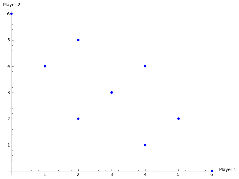
Consider the following stage game:

$\begin{pmatrix} (2,3)&(0,2)&(1,4)\\ (0,1)&(1,2)&(0,0)\\ \end{pmatrix}$

The plot shows the various possible outcomes of the repeated game for $T=2$.

$All possible outcomes of the repeated $3\times2$ game.\label{L09-plot02}$

If we consider the two pure equilibria $(r_1,c_3)$ and $(r_2,c_2)$, we have 4 possible outcomes that correspond to the outcome of a subgame perfect Nash equilibria:

$(r_1r_1,c_3c_3)\text{ giving utility vector: }(2,8)$ $(r_1r_2,c_3c_2)\text{ giving utility vector: }(2,6)$ $(r_2r_1,c_2c_3)\text{ giving utility vector: }(2,6)$ $(r_2r_2,c_2c_2)\text{ giving utility vector: }(2,4)$

Importantly, not all subgame Nash equilibria outcomes are of the above form.

Reputation in repeated games

By definition all subgame Nash equilibria must play a stage Nash profile in the last stage game. However can a strategy be found that does not play a Nash profile in earlier games?

Considering the above game, let us look at this strategy:

“Play $(r_1,c_1)$ in the first period and then, as long as P2 cooperates play $(r_1,c_3)$ in the second period. If P2 deviates from $c_1$ in the first period then play $(r_2,c_2)$ in the second period.”

Firstly this strategy gives the utility vector: $(3,7)$.

Is this strategy profile a Nash equilibrium (for the entire game)?

Does player 1 have an incentive to deviate?

No any other strategy played in any period would give a lower payoff.

Does player 2 have an incentive to deviate?

If player 2 deviates in the first period, he/she can obtain 4 in the first period but will obtain 2 in the second. Thus a first period deviation increases the score by 1 but decreases the score in the second period by 2. Thus player 2 does not have an incentive to deviate.

Finally to check that this is a subgame perfect Nash equilibrium we need to check that it is an equilibrium for the whole game as well as all subgames.

We have checked previously that it is an equilibrium for the entire game.
It is also subgame perfect as the profile dictates a stage Nash profile in the last stage.

Chapter 10 - Infinitely Repeated Games

Recap

In the previous chapter:

We defined repeated games;
We showed that a sequence of stage Nash games would give a subgame perfect equilibria;
We considered a game, illustrating how to identify equilibria that are not a sequence of stage Nash profiles.

In this chapter we’ll take a look at what happens when games are repeatedly infinitely.

Discounting

To illustrate infinitely repeated games ($T\to\infty$) we will consider a Prisoners dilemma as our stage game.

$\begin{pmatrix} (2,2)&(0,3)\\ (3,0)&(1,1) \end{pmatrix}$

Let us denote $s_{C}$ as the strategy “cooperate at every stage”. Let us denote $s_{D}$ as the strategy “defect at every stage”.

If we assume that both players play $s_{C}$ their utility would be:

$U_1(s_{C},s_{C})=U_2(s_{C},s_{C})=\sum_{t=1}^\infty2>\infty$

Similarly:

$U_1(s_{D},s_{D})=U_2(s_{D},s_{D})=\sum_{t=1}^\infty1>\infty$

It is impossible to compare these two strategies. To be able to carry out analysis of strategies in infinitely repeated games we make use of a discounting factor $0<\delta<1$.

The interpretation of $\delta$ is that there is less importance given to future payoffs. One way of thinking about this is that “the probability of recieveing the future payoffs decreases with time”.

In this case we write the utility in an infinitely repeated game as:

$U_i(r,c)=\sum_{t=1}^\infty\delta^{t-1}u_i(r(t),c(t))$

Thus:

$U_1(s_{C},s_{C})=U_2(s_{C},s_{C})=2\sum_{t=1}^\infty\delta^{t-1}=2/(1-\delta)$

and:

$U_1(s_{D},s_{D})=U_2(s_{D},s_{D})=\sum_{t=1}^\infty\delta^{t-1}=1/(1-\delta)$

Conditions for cooperation in Prisoner’s Dilemmas

Let us consider the “Grudger” strategy (which we denote $s_G$):

“Start by cooperating until your opponent defects at which point defect in all future stages.”

If both players play $s_G$ we have $s_G=s_C$:

$U_1(s_{G},s_{G})=U_2(s_{G},s_{G})=2/(1-\delta)$

If we assume that $S_1=S_2=\{s_C,s_D,s_G\}$ and player 2 deviates from $S_G$ at the first stage to $s_D$ we get:

$U_2(s_{G},s_{D})=3+\sum_{t=2}^{\infty}\delta^{t-1}=3+\delta/(1-\delta)$

Deviation from $s_G$ to $s_D$ is rational if and only if:

$2/(1-\delta)<3+\delta/(1-\delta)$ $\Leftrightarrow$ $\delta< 1/2$

thus if $\delta$ is large enough $(s_G,s_G)$ is a Nash equilibrium.

Importantly $(s_G,s_G)$ is not a subgame perfect Nash equilibrium. Consider the subgame following $(r_1,c_2)$ having been played in the first stage of the game. Assume that player 1 adhers to $s_G$:

If player 2 also plays $s_G$ then the first stage of the subgame will be $(r_2,c_1)$ (player 1 punishes while player 2 sticks with $c_1$ as player 1 played $r_1$ in previous stage). All subsequent plays will be $(r_2,c_2)$ so player 2’s utility will be:
$0+\sum_{t=2}^{\infty}\delta^{t-1}=\delta/(1-\delta)$
If player 2 deviates from $s_G$ and chooses to play $D$ in every period of the subgame then player 2’s utility will be:
$\sum_{t=1}^{\infty}\delta^{t-1}=1/(1-\delta)$

which is a rational deviation (as $0<\delta<1$).

Two questions arise:

Can we always find a strategy in a repeated game that gives us a better outcome than simply repeating the stage Nash equilibria? (Like $s_G$)
Can we also find a strategy with the above property that in fact is subgame perfect? (Unlike $s_G$)

Folk theorem

The answer is yes! To prove this we need to define a couple of things.

Definition of an average payoff

If we interpret $\delta$ as the probability of the repeated game not ending then the average length of the game is:

$\bar T=\frac{1}{1-\delta}$

We can use this to define the average payoffs per stage:

$\frac{1}{\bar T}U_i(r,c)=(1-\delta)U_i(r,c)$

This average payoff is a tool that allows us to compare the payoffs in an infitely repeated game to the payoff in a single stage game.

Definition of individually rational payoffs

Individually rational payoffs are average payoffs that exceed the stage game Nash equilibrium payoffs for both players.

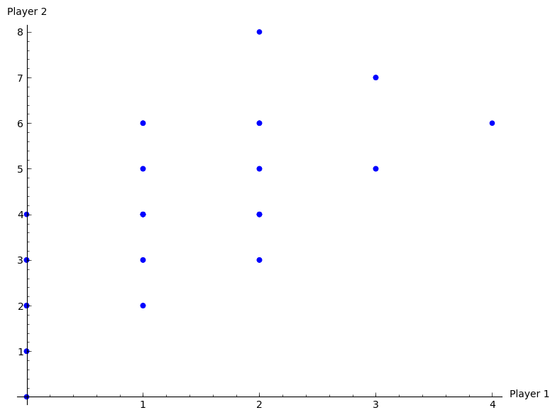
As an example consider the plot corresponding to a repeated Prisoner’s Dilemma.

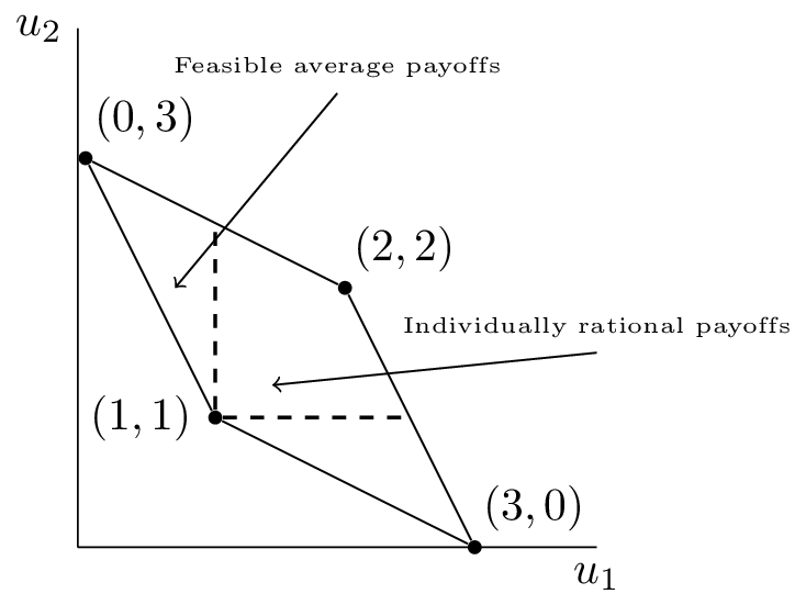
$Convex hull of payoffs to a prisoners dilemma.\label{L10-img01}$

The feasible average payoffs correspond to the feasible payoffs in the stage game. The individually rational payoffs show the payoffs that are better for both players than the stage Nash equilibrium.

The following theorem states that we can choose a particular discount rate that for which there exists a subgame perfect Nash equilibrium that would give any individually rational payoff pair!

Folk Theorem for infinitely repeated games

Let $(u_1^*,u_2^*)$ be a pair of Nash equilibrium payoffs for a stage game. For every individually rational pair $(v_1,v_2)$ there exists $\bar \delta$ such that for all $1>\delta>\bar \delta>0$ there is a subgame perfect Nash equilibrium with payoffs $(v_1,v_2)$.

Proof

Let $(\sigma_1^*,\sigma_2^*)$ be the stage Nash profile that yields $(u_1^*,u_2^*)$. Now assume that playing $\bar\sigma_1\in\Delta S_1$ and $\bar\sigma_2\in\Delta S_2$ in every stage gives $(v_1,v_2)$ (an individual rational payoff pair).

Consider the following strategy:

“Begin by using $\bar \sigma_i$ and continue to use $\bar \sigma_i$ as long as both players use the agreed strategies. If any player deviates: use $\sigma_i^*$ for all future stages.”

We begin by proving that the above is a Nash equilibrium.

Without loss of generality if player 1 deviates to $\sigma_1’\in\Delta S_1$ such that $u_1(\sigma_1’,\bar \sigma_2)>v_1$ in stage $k$ then:

$U_1^{(k)}=\sum_{t=1}^{k-1}\delta^{t-1}v_1+\delta^{k-1}u_1(\sigma_1',\bar \sigma_2)+u_1^*\left(\frac{1}{1-\delta}-\sum_{t=1}^{k}\delta^{t-1}\right)$

Recalling that player 1 would receive $v_1$ in every stage with no devitation, the biggest gain to be made from deviating is if player 1 deviates in the first stage (all future gains are more heavily discounted). Thus if we can find $\bar\delta$ such that $\delta>\bar\delta$ implies that $U_1^{(1)}\leq \frac{v_1}{1-\delta}$ then player 1 has no incentive to deviate.

$\begin{aligned} U_1^{(1)}=u_1(\sigma_1',\bar\sigma_2)+u_1^*\frac{\delta}{1-\delta}&\leq\frac{v_1}{1-\delta}\\ (1-\delta)u_1(\sigma_1',\bar\sigma_2)+u_1^*\delta&\leq v_1\\ u_1(\sigma_1',\bar\sigma_2)-v_1&\leq \delta(u_1(\sigma_1',\bar\sigma_2)-u_1^*)\\ \end{aligned}$

as $u_1(\sigma_1’,\bar \sigma_2)>v_1>u_1^*$, taking $\bar\delta=\frac{u_1(\sigma_1’,\bar\sigma_2)-v_1}{u_1(\sigma_1’,\bar\sigma_2)-u_1^*}$ gives the required required result for player 1 and repeating the argument for player 2 completes the proof of the fact that the prescribed strategy is a Nash equilibrium.

By construction this strategy is also a subgame perfect Nash equilibrium. Given any history both players will act in the same way and no player will have an incentive to deviate:

If we consider a subgame just after any player has deviated from $\bar\sigma_i$ then both players use $\sigma_i^*$.
If we consider a subgame just after no player has deviated from $\bar\sigma_i$ then both players continue to use $\bar\sigma_i$.

Chapter 11 - Population Games and Evolutionary stable strategies

Recap

In the previous chapter

We considered infinitely repeated games using a discount rate;
We proved a powerful result stating that for a high enough discount rate player would cooperate.

In this chapter we’ll start looking at a fascinating area of game theory.

Population Games

In this chapter (and the next) we will be looking at an area of game theory that looks at the evolution of strategic behaviour in a population.

Definition of a population vector

Considering an infinite population of individuals each of which represents a strategy from $\Delta S$, we define the population profile as a vector $\chi\in[0,1]^{|S|}_\mathbb{R}$. Note that:

$\sum_{s\in S}\chi(s)=1$

It is important to note that $\chi$ does not necessarily correspond to any strategy adopted by particular any individual.

Example

Consider a population with $S=\{s_1,s_2\}$. If we assume that every individual plays $\sigma=(.25,.75)$ then $\chi=\sigma$. However if we assume that .25 of the population play $\sigma_1=(1,0)$ and .75 play $\sigma_2=(0,1)$ then $\chi=\sigma$.

In evolutionary game theory we must consider the utility of a particular strategy when played in a particular population profile denoted by $u(s,\chi)$ for $s\in S$.

Thus the utility to a player playing $\sigma\in\Delta S$ in a population $\chi$:

$u(\sigma,\chi)=\sum_{s\in S}\sigma(s)u(s,\chi)$

The interpretation of the above is that these payoffs represent the number of descendants that each type of individual has.

Example

If we consider a population of N individuals in which $S=\{s_1,s_2\}$. Assume that .5 of the population use each strategy so that $\chi=(.5,.5)$ and assume that for the current population profile we have:

$u(s_1,\chi)=3\text{ and }u(s_2,\chi)=7$

In the next generation we will have $3N/2$ individuals using $s_1$ and $7N/2$ using $s_2$ so that the strategy profile of the next generation will be $(.3,.7)$.

We are going to work towards understanding the evolutionary dynamics of given populations. If we consider $\chi$ to be the startegy profile where all members of the population play $\sigma^*$ then a population will be stable only if:

$\sigma^*\in\text{argmax}_{\sigma\in\Delta S}u(\sigma,\chi)$

Ie at equilibrium $\sigma^*$ must be a best response to the population profile it generates.

Theorem for necessity of stability

In a population game, consider $\sigma^*\in\Delta S$ and the population profile $\chi$ generated by $\sigma^*$. If the population is stable then:

$u(s,\chi)=u(\sigma^*,\chi)\text{ for all }s\in\mathcal{S}(\sigma^*)$

(Recall that $\mathcal{S}(s)$ denotes the support of $s$.)

Proof

If $|\mathcal{S}(\sigma^*)|=1$ then the proof is trivial.

We assume that $|\mathcal{S}(\sigma^*)|>1$. Let us assume that the theorem is not true so that there exists $\bar s\in\mathcal{S}(\sigma^*)$ such that:

$u(\sigma^*,\chi)\ne u(\bar s,\chi)$

Without loss of generality let us assume that:

$\bar s=\text{argmax}_{s\in\mathcal{S}(\sigma^*)}u(s,\chi)$

Thus we have:

$\begin{aligned} u(\sigma^*,\chi)&=\sum_{s\in\mathcal{S}(\sigma^*)}\sigma^*(s)u(s,\chi)\\ &\leq\sum_{s\in\mathcal{S}(\sigma^*)}\sigma^*(s)u(\bar s,\chi) \\ &\leq u(\bar s,\chi)\sum_{s\in\mathcal{S}(\sigma^*)}\sigma^*(s) \\ &\leq u(\bar s,\chi) \end{aligned}$

Which gives:

$u(\sigma^*,\chi)< u(\bar s,\chi)$

which implies that the population is not stable.

Evolutionary Stable Strategies

Definition of an evolutionary stable strategy

Consider a population where all individuals initially play $\sigma^*$. If we assume that a small proportion $\epsilon$ start playing $\sigma$. The new population is called the post entry population and will be denoted by $\chi_{\epsilon}$.

Example

Consider a population with $S=\{s_1,s_2\}$ and initial population profile $\chi=(1/2,1/2)$. If we assume that $\sigma=(1/3,2/3)$ is introduced in to the population then:

$\begin{aligned} \chi_{\epsilon}&=(1-\epsilon)(1/2,1/2)+\epsilon\sigma\\ &=(1/2-\epsilon/6,1/2+\epsilon/6) \end{aligned}$

Definition

A strategy $\sigma^*\in\Delta S$ is called an Evolutionary Stable Strategy if there exists an $0<\bar\epsilon<1$ such that for every $0<\epsilon<\bar \epsilon$ and every $\sigma\ne \sigma^*$:

$u(\sigma^*,\chi_\epsilon)>u(\sigma,\chi_\epsilon)$

Before we go any further we must consider two types of population games:

Games against the field. In this setting we assume that no individual has a specific adversary but has a utility that depends on what the rest of the individuals are doing.
Pairwise contest games. In this setting we assume that every individual is continiously assigned to play against another individual.

The differences between these two types of population games will hopefully become clear.

Games against the field

We will now consider an example of a game against the field. The main difficulty with these games is that the utility $u(s,\chi)$ is not generally linear in $\chi$.

Let us consider the Male to Female ratio in a population, and make the following assumptions:

The proportion of Males in the population is $\alpha$ and the proportion of females is $1-\alpha$;
Each female has a single mate and has $K$ offspring;
Males have on average $(1-\alpha)/\alpha$ mates;
Females are solely responsible for the sex of the offspring.

We assume that $S=\{M,F\}$ so that females can either only produce Males or only produce Females. Thus, a general mixed strategy $\sigma=(\omega,1-\omega)$ produces a population with a proportion of $\omega$ males. Furthermore we can write $\chi=(\alpha,1-\alpha)$.

The females are the decision makers so that we consider them as the individuals in our population. The immediate offspring of the females $K$ is constant and so cannot be used as a utility. We use the second generation offspring:

$\begin{aligned} u(M,\chi)&=K^2\frac{1-\alpha}{\alpha}\\ u(F,\chi)&=K^2 \end{aligned}$

Thus:

$u(\sigma,\chi)=K^2\left(\omega\frac{(1-\alpha)}{\alpha}+(1-\omega)\right)$

Note that we can assume that $K=1$ for the rest of this exercise as we will ultimately be comparing different values of the utility.

Let us try and find an ESS for this game:

If $\alpha\ne 1/2$ then $u(M,\chi)\ne u(F,\chi)$ so that any mixed strategy $\sigma$ with support ${M,F}$ would not give a stable population.
Thus we need to check if $\sigma^*=(1/2,1/2)$ is an ESS (this is the only candidate).

We consider some mutation $\sigma=(p,1-p)$:

$\chi_{\epsilon}=(1-\epsilon)\sigma^*+\epsilon\sigma$

which implies that the proportion of population playing $M$ in $\chi_{\epsilon}$ is given by:

$\alpha_{\epsilon}=(1-\epsilon)1/2+p\epsilon=1/2+\epsilon(p-1/2)$

We have:

$u(\sigma^*,\chi_{\epsilon})=1/2+\frac{1-\alpha_{\epsilon}}{2\alpha_{\epsilon}}$

and:

$u(\sigma,\chi_{\epsilon})=(1-p)+p\frac{1-\alpha_{\epsilon}}{\alpha_{\epsilon}}$

The difference:

$\begin{aligned} u(\sigma^*,\chi_{\epsilon})-u(\sigma,\chi_{\epsilon})&=p-1/2+(1/2-p)\frac{1-\alpha_{\epsilon}}{\alpha_{\epsilon}}\\ &=(1/2-p)\frac{1-2\alpha_{\epsilon}}{\alpha_{\epsilon}} \end{aligned}$

We note that if $p<1/2$ then $\alpha_{\epsilon}<1/2$ which implies that $u(\sigma^*,\chi_{\epsilon})-u(\sigma,\chi_{\epsilon})>0$. Similarly if $p>1/2$ then $\alpha_{\epsilon}>1/2$ which implies that $u(\sigma^*,\chi_{\epsilon})-u(\sigma,\chi_{\epsilon})>0$. Thus $\sigma^*=(1/2,1/2)$ is a ESS.

Chapter 12 - Nash equilibrium and Evolutionary stable strategies

Recap

In the previous chapter:

We considered population games;
We proved a result concerning a necessary condition for a population to be evolutionary stable;
We defined Evolutionary stable strategies and looked at an example in a game against the field.

In this chapter we’ll take a look at pairwise contest games and look at the connection between Nash equilibrium and ESS.

Pairwise contest games

In a population game when considering a pairwise contest game we assume that individuals are randomly matched. The utilities then depend just on what the individuals do:

$u(\sigma,\chi)=\sum_{s\in S}\sum_{s'\in S}\sigma(s)\chi(s')u(s,s')$

As an example we’re going to consider the “Hawk-Dove” game: a model of predator interaction. We have $S={H,D}$ were:

$H$: Hawk represents being “aggressive”;
$D$: Dove represents not being “aggressive”.

At various times individuals come in to contact and must choose to act like a Hawk or like Dove over the sharing of some resource of value $v$. We assume that:

If a Dove and Hawk meet the Hawk takes the resources;
If two Doves meet they share the resources;
If two Hawks meet there is a fight over the resources (with an equal chance of winning) and the winner takes the resources while the loser pays a cost $c>v$.

If we assume that $\sigma=(\omega,1-\omega)$ and $\chi=(h,1-h)$ the above gives:

$u(\sigma,\chi)=\omega(1-h)v+(1-\omega)(1- h) \frac{v}{2}+\omega h \frac{v-c}{2}$

It is immediate to note that no pure strategy ESS exists. In a population of Doves ($h=0$):

$u(\sigma,(0,1))=\omega v+(1-\omega) \frac{v}{2}=(1+\omega)\frac{v}{2}$

thus the best response is setting $\omega=1$ i.e. to play Hawk.

In a population of Hawks ($h=1$):

$u(\sigma,(1,0))=\omega \frac{v-c}{2}$

thus the best response is setting $\omega=0$ i.e. to play Dove.

So we will now try and find out if there is a mixed-strategy ESS: $\sigma^*=(\omega^*,1-\omega^*)$. For $\sigma^*$ to be an ESS it must be a best response to the population it generates $\chi^*=(\omega^*,1-\omega^*)$. In this population the payoff to an arbitrary strategy $\sigma$ is:

$u(\sigma,\chi^*)=(1-\omega^*)\frac{v}{2}+\left(\frac{v}{c}-\omega^*\right)\frac{\omega c}{2}$

If $\omega^*<v/c$ then a best response is $\omega=1$;
If $\omega^*>v/c$ then a best response is $\omega=0$;
If $\omega^*=v/c$ then there is indifference.

So the only candidate for an ESS is $\sigma^*=\left(v/c,1-v/c\right)$. We now need to show that $u(\sigma^*,\chi_{\epsilon})>u(\sigma,\chi_{\epsilon})$.

We have:

$x_\epsilon=(v/c+\epsilon(\omega-v/c),1-v/c+\epsilon(v/c-\omega)$

and:

$\begin{aligned} u(\sigma^*,\chi_{\epsilon})=\frac{v}{c}\left(\frac{v}{c}+\epsilon\left(\omega-\frac{v}{c}\right)\right)\frac{v-c}{2}+&\frac{v}{c}\left(1-\frac{v}{c}+\epsilon\left(\frac{v}{c}-\omega\right)\right)v\\ +&\left(1-\frac{v}{c}\right)\left(1-\frac{v}{c}+\epsilon\left(\frac{v}{c}-\omega\right)\right)\frac{v}{2} \end{aligned}$ $\begin{aligned} u(\sigma,x_{\epsilon})=\omega\left(\frac{v}{c}+\epsilon\left(\omega-\frac{v}{c}\right)\right)\frac{v-c}{2}+&\omega\left(1-\frac{v}{c}+\epsilon\left(\frac{v}{c}-\omega\right)\right)v\\ +&\left(1-\omega\right)\left(1-\frac{v}{c}+\epsilon\left(\frac{v}{c}-\omega\right)\right)\frac{v}{2} \end{aligned}$

This gives:

$u(\sigma^*,\chi_{\epsilon})-u(\sigma,x_{\epsilon})=\frac{\epsilon c}{2}\left(\frac{v}{c}-\omega\right)^2>0$

which proves that $\sigma^*$ is an ESS.

We will now take a closer look the connection between ESS and Nash equilibria.

ESS and Nash equilibria

When considering pairwise contest population games there is a natural way to associate a normal form game.

Definition

The associated two player game for a pairwise contest population game is the normal form game with payoffs given by: $u_1(s,s’)=u(s,s’)=u_2(s’,s)$.

Note that the resulting game is symmetric (other contexts would give non symmetric games but we won’t consider them here).

Using this we have the powerful result:

Theorem relating an evolutionary stable strategy to the Nash equilibrium of the associated game

If $\sigma^*$ is an ESS in a pairwise contest population game then for all $\sigma\ne\sigma^*$:

$u(\sigma^*,\sigma^*)>u(\sigma,\sigma^*)$ OR
$u(\sigma^*,\sigma^*)=u(\sigma,\sigma^*)$ and $u(\sigma^*,\sigma)>u(\sigma,\sigma)$

Conversely, if either (1) or (2) holds for all $\sigma\ne\sigma^*$ in a two player normal form game then $\sigma^*$ is an ESS.

Proof

If $\sigma^*$ is an ESS, then by definition:

$u(\sigma^*,\chi_{\epsilon})>u(\sigma,\chi_{\epsilon})$

which corresponds to:

$(1-\epsilon)u(\sigma^*,\sigma^*)+\epsilon u(\sigma^*,\sigma)>(1-\epsilon)u(\sigma,\sigma^*)+\epsilon u(\sigma,\sigma)$

If condition 1 of the theorem holds then the above inequality can be satisfied for $\epsilon$ sufficiently small. If condition 2 holds then the inequality is satisfied.
Conversely:
- If $u(\sigma^*,\sigma^*)<u(\sigma,\sigma^*)$ then we can find $\epsilon$ sufficiently small such that the inequality is violated. Thus the inequality implies $u(\sigma^*,\sigma^*)\geq u(\sigma,\sigma^*)$.
- If $u(\sigma^*,\sigma^*)= u(\sigma,\sigma^*)$ then $u(\sigma^*,\sigma)> u(\sigma,\sigma)$ as required.

This result gives us an efficient way of computing ESS. The first condition is in fact almost a condition for Nash Equilibrium (with a strict inequality), the second is thus a stronger condition that removes certain Nash equilibria from consideration. This becomes particularly relevant when considering Nash equilibrium in mixed strategies.

To find ESS in a pairwise context population game we:

Write down the associated two-player game;
Identify all symmetric Nash equilibria of the game;
Test the Nash equilibrium against the two conditions of the above Theorem.

Example

Let us consider the Hawk-Dove game. The associated two-player game is:

$\begin{pmatrix} \left(\frac{v-c}{2},\frac{v-c}{2}\right),(v,0)\\ (0,v),\left(\frac{v}{2},\frac{v}{2}\right)\\ \end{pmatrix}$

Recalling that we have $v<c$ so we can use the Equality of payoffs theorem to obtain the Nash equilibrium:

$\begin{aligned} u_2(\sigma^*,H)&= u_2(\sigma^*,D)\\ q^*&=\frac{v}{c} \end{aligned}$

Thus we will test $\sigma^*=(\frac{v}{c},1-\frac{v}{c})$ using the above theorem.

Importantly from the equality of payoffs theorem we immediately see that condition 1 does not hold as $u(\sigma^*,\sigma^*)=u(\sigma^*,H)=u(\sigma^*,D)$. Thus we need to prove that:

$u(\sigma^*,\sigma)>u(\sigma,\sigma)$

We have:

$u(\sigma^*,\sigma)=\frac{v}{c}\omega\frac{v-c}{2}+\frac{v}{c}(1-\omega)v+(1-\frac{v}{c})(1-\omega)\frac{v}{2}$ $u(\sigma,\sigma)=\omega^2\frac{v-c}{2}+\omega(1-\omega)v+(1-\omega)^2\frac{v}{2}$

After some algebra:

$u(\sigma^*,\sigma)-u(\sigma,\sigma)=\frac{c}{2}(\frac{v}{c}-\omega)^2>0$

Giving the required result.

Chapter 13 - Random events and incomplete information

Recap

In the previous chapter:

We considered pairwise contest population games;
We proved a result showing the connection between ESS and NE.

In this chapter we will take a look at how to model games with incomplete information and random events.

Representing incomplete information in extensive form games

Game with incomplete information represent situations where the players do not possess exact knowledge of the environment. This is represented by associating probabilities to various states. We show this on game trees using red circles to represent decisions made by “nature” where we can consider “nature” as a player although not a strategic one.

If we recall the first game tree we considered in Chapter 1 we had already done this to some extent.

$A 1 player game with incomplete information.\label{L01-img01}$

Let us consider a slightly more complicated game.

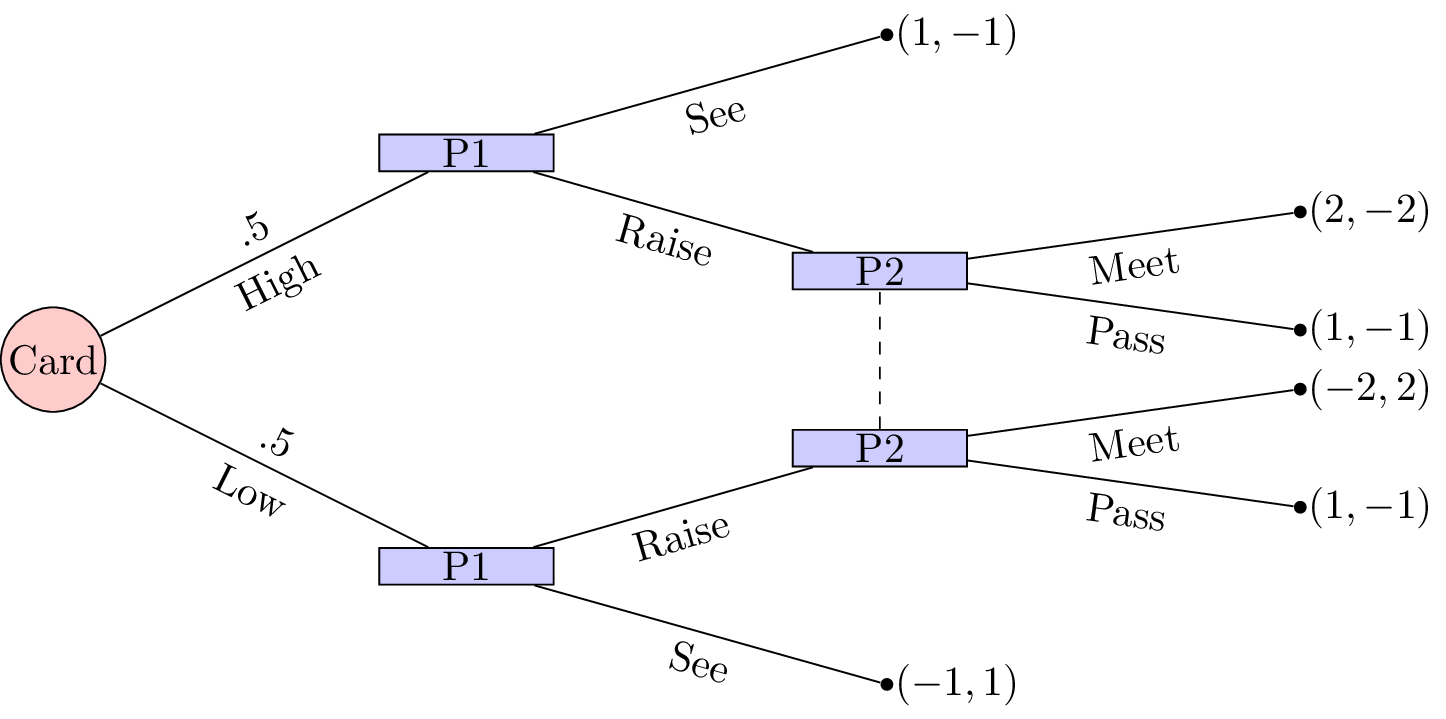
“Two players play a card game. They each put a dollar in a pot. Player 1 is dealt a card that is either high or low with equal probability. Player1 observes the card but player 2 does not. Player 1 may see or raise. If player 1 sees then the card is shown and player 1 takes the dollar if the card if high or player 2 takes the dollar. If player 1 raises, player 1 adds a dollar to the pot. Player 2 can then pass or meet. If player 2 passes then player 1 takes the pot. Otherwise, player 2 adds a dollar to the pot. If player 1’s card is high then player 1 takes the pot else player 2 takes the pot.”

This game is represented shown.

$A simplified game of poker.\label{L13-img01}$

To solve this game we can (as in Chapter 8) obtain the corresponding normal form game by taking expected utilities over the moves of nature.

We have $S_1=\{\text{SeeRaise},\text{SeeSee},\text{RaiseRaise},\text{RaiseSee}\}$ and $S_2=\{\text{Meet},\text{Pass}\}$ and the normal form representation is:

$\begin{pmatrix} (-1/2,1/2)&(1,-1)\\ (0,0)&(0,0)\\ (0,0)&(1,-1)\\ (1/2,-1/2)&(0,0) \end{pmatrix}$

In this game we see that $\text{SeeSee}$ is dominated by any mixed strategy with support: $\{\text{RaiseRaise},\text{RaiseSee}\}$. Similarly $\text{SeeRaise}$ is not a best response to any strategy of player 2 that plays $\text{Meet}$ with non zero probability. Thus we have $\sigma_1=(0,0,x,1-x)$. Using the equality of payoffs theorem we have:

$\begin{aligned} u_2(\sigma_1,\text{Meet})&=u_2(\sigma_1,\text{Pass})\\ (x-1)/2&=-x\\ x&=1/3 \end{aligned}$

Using the Equality of Payoffs theorem we get that the Nash equilibrium is $\sigma_1=(0,0,1/3,2/3)$ and $\sigma_2=(2/3,1/3)$. I.e. player 1 should always raise if the card is high and bluff with probability $1/3$ if the card is low.

Utilities

When considering games with uncertainty it is particularly relevant to consider some basic utility theory. Consider the following game shown.

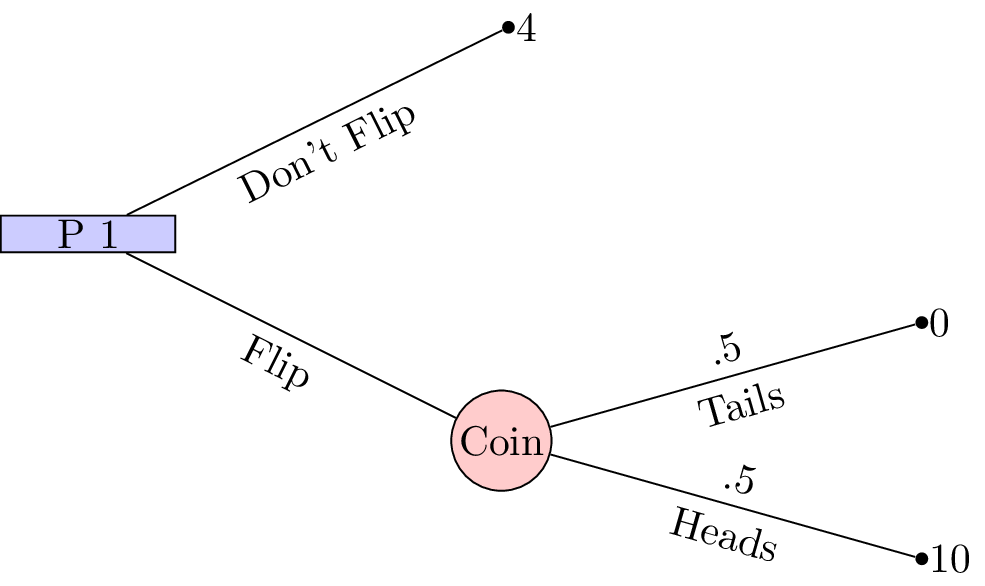
$A simple 1 player game with incomplete information.\label{L13-img02}$

This is a 1 player game where a player must choose whether or not to flip a coin. If the coin is flipped and lands on “Heads” then the player wins £10, if the coin lands on “Tails” then the player wins nothing. If the player chooses to not flip a coin then the player wins £4.

With such small sums of money involved it is quite likely that the player would choose to flip the coin (afterall the expected value of flipping the coin is £5. If we changed the game slightly so that it was now in terms of millions of pounds surely the player should just take the £4 million on offer?

This perception is due to the fact that the percieved gain from 0 to £4 million is much larger than the percieved gain from £4 million to £10 million. This can be modelled mathematically using convex and concave functions:

“Risk averse”: a concave utility function.
“Risk neutral”: a linear function.
“Risk seeking”: a convex function.

This is shown.

$Utility function. \label{L13-plot01}$

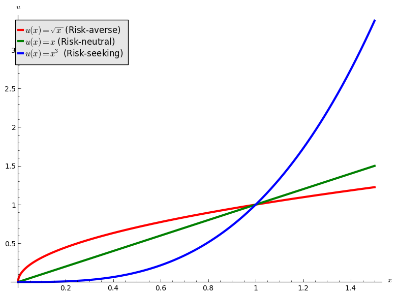
If we use $u=\sqrt{x}$ as the utility function in the coin flip game we see that the analytical solution would indeed be to not flip. We will now take a look at this in a bit more detail with a well known game.

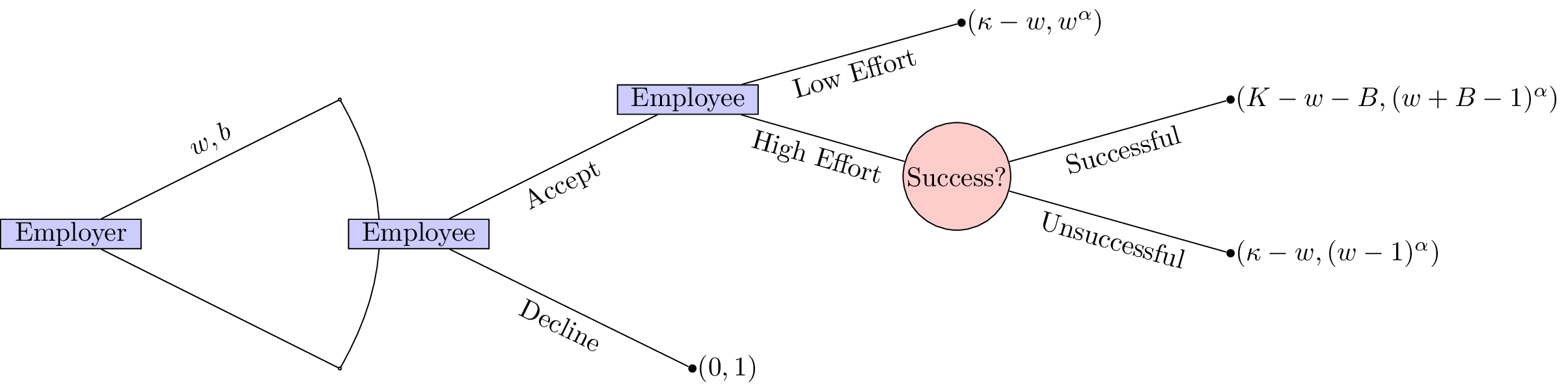
Principal agent game

Consider a game with two players. The first player is an employer and the second a potential employee. The employer must decide on two parameters:

A wage value: $w$;
A bonus value: $B$.

The potential employee must then make two decisions:

Whether or not to accept the job;
If the job is accepted to either put in a high level of effort or a low level of effort.

The success of the project that requires the employee is as follows:

If the employee puts in a high level of effort the project will be succesful with probability $1/2$;
If the employee puts in a low level of effort the project will be unsussesful.

The monetary gain to the employer is as follows:

If the employee does not take the job the utility is 0.
If the project is succesful: $K$;
If the project is unsuccesful: $\kappa$.

The monetary gain to the employee is as follows:

If the job offer is not accepted: 1;
If the project is succesful: $w+B-1$ (the lost gain corresponds to the effort);
If the project is unsuccesful despite a high level of effort: $w-1$ (the lost gain corresponds to the effort), we assume that $w\geq 1$;
If the project is unsuccesful because of a low level of effort: $w$.

We furthermore assume that the utility function of the employer is simply $u(x)=x$ while the utility function to the potential employee is of the form $u(x)=x^{\alpha}$ for $0<\alpha<1$ (i.e. the potential employee is risk averse).

The extensive form of the game is shown.

$The principal agent game.\label{L13-img03}$

Immediately we see that this game is trivial if $\kappa<\omega$ and $K<\omega+B$. Furthermore it seems sensible to only consider $K>\kappa$.

We will solve this game using backward induction. The first step is shown.

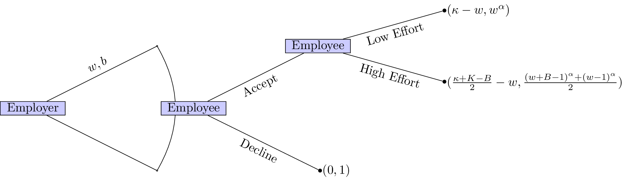
$Calculating the expected value of move by nature. \label{L13-img04}$

If the employer would like a high level of effort he should set $w,B$ such that:

$\frac{(w+B-1)^\alpha+(w-1)^\alpha}{2}\geq w^\alpha$

This ensures that the employee will put in a high level of effort. Furthermore it is in the employers interest to ensure that the employee accepts the job (we assume here that $\frac{\kappa+K+B}{2}\geq w$):

$\frac{(w+B-1)^\alpha+(w-1)^\alpha}{2}\geq 1$

This second inequality ensures that the employee accepts the position. Given that the position is accepted the employer would like to in fact minimise $w,B$ thus we have:

$\frac{(w+B-1)^\alpha+(w-1)^\alpha}{2}=1$

Thus we have:

$w^\alpha\leq 1$

however we assume that $w\geq 1$ (so that the “wage is worth the effort”) so we in fact have $w=1$. This then gives: $B=2^{1/\alpha}$. The expected utilities are then:

Employer: $\frac{\kappa+K-2^{1/\alpha}}{2}-1$;
Employee: 1.

Note that the employer’s utility is an increasing function in $\alpha$. As the potential employee becomes more and more risk neutral the employer does not need to offer a high bonus to incite a high level of effort.

Chapter 14 - Stochastic games

Recap

In the previous chapter:

We considered games of incomplete information;
Discussed some basic utility theory;
Considered the principal agent game.

In this chapter we will take a look at a more general type of random game.

Stochastic games

Definition of a stochastic game

A stochastic game is defined by:

X a set of states with a stage game defined for each state;
A set of strategies $S_i(x)$ for each player for each state $x\in X$;
A set of rewards dependant on the state and the actions of the other players: $u_i(x,s_1,s_2)$;
A set of probabilities of transitioning to a future state: $\pi(x’|x,s_1,s_2)$;
Each stage game is played at a set of discrete times $t$.

We will make some simplifying assumptions in this course:

The length of the game is not known (infinite horizon) - so we use discounting;
The rewards and transition probabilities are not dependent;
We will only consider strategies called Markov strategies.

Definition of a Markov strategy

A strategy is call a Markov strategy if the behaviour dictated is not time dependent.

Example

Consider the following game with $X=\{x,y\}$:

$S_1(x)=\{a,b\}$ and $S_2(x)=\{c,d\}$;
$S_1(y)=\{e\}$ and $S_2(x)=\{f\}$;

We have the stage game corresponding to state $x$:

$\begin{pmatrix} (8,4)&(5,3)\\ (1,5)&(2,6) \end{pmatrix}$

The stage game corresponding to state $y$:

$\begin{pmatrix} (0,0)\\ \end{pmatrix}$

The transition probabilities corresponding to state $x$:

$\begin{pmatrix} (.5,.5)&(1,0)\\ (1,0)&(1,0) \end{pmatrix}$

The transition probabilities corresponding to state $y$:

$\begin{pmatrix} (0,1)\\ \end{pmatrix}$

A concise way of representing all this is shown.

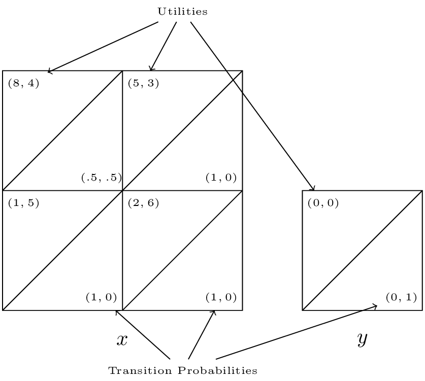
$A simple stochastic game.\label{L14-img01}$

We see that the Nash equilibrium for the stage game corresponding to $x$ is $(a, c)$ however as soon as the players play that strategy profile they will potentially go to state $y$ which is an absorbing state at which players gain no further utility.

To calculate utilities for players in infinite horizon stochastic games we use a discount rate. Thus without loss of generality if the game is in state $x$ and we assume that both players are playing $\sigma^*_i$ then player 1 would be attempting to maximise future payoffs:

$U_1(r,c)=\left(u_1(x,r,c)+\delta\sum_{x'\in X}\pi(x'|x,r,c)U_1^*(x')\right)$

where $U_1^*$ denotes the expected utility to player 1 when both players are playing the Nash strategy profile.

Thus a Nash equilibrium satisfies:

$U_1^*(x)=\max_{r\in S_1(x)}(u_i(x,r,c^* )+\delta\sum_{x'\in X}\pi(x'|x,r,c^*)U_1^*(x'))$ $U_2^*(x)=\max_{c\in S_2(x)}(u_i(x,r^*,c)+\delta\sum_{x'\in X}\pi(x'|x,r^*,c)U_2^*(x'))$

Solving these equations is not straightforward. We will take a look at one approach by solving the example we have above.

Finding equilibria in stochastic games

Let us find a Nash equilibrium for the game considered above with $\delta=2/3$.

State $y$ gives no value to either player so we only need to consider state $x$. Let the future gains to player 1 in state $x$ be $v$, and the future gains to player 2 in state $x$ be $u$. Thus the players are facing the following game:

$\begin{pmatrix} (8+\frac{1}{3}v,4+\frac{1}{3}u)&(5+\frac{2}{3}v,3+\frac{2}{3}u)\\ (1+\frac{2}{3}v,5+\frac{2}{3}u)&(2+\frac{2}{3}v,6+\frac{2}{3}u) \end{pmatrix}$

We consider each strategy pair and state the condition for Nash equilibrium:

$(a,c)$: $v\leq 21$ and $u\leq 3$.
$(a,d)$: $u\geq3$.
$(b,c)$: $v\geq 21$ and $5\geq 6$.
$(b,d)$: $5\leq2$.

Now consider the implications of each of those profiles being an equilibrium:

$8+v/3=v$ $\Rightarrow$ $v=12$ and $4+u/3=u$ $\Rightarrow$ $u=6$ which contradicts the corresponding inequality.
$3+2u/3=u$ $\Rightarrow$ $u=9$.
The second inequality cannot hold.
The inequality cannot hold.

Thus the unique Markov strategy Nash equilibria is $(a,d)$ which is not the stage Nash equilibria!

Chapter 15 - Matching games

Recap

In the previous chapter:

We defined stochastic games;
We investigated approached to obtaining Markov strategy Nash equilibria.

In this chapter we will take a look at a very different type of game.

Matching Games

Consider the following situation:

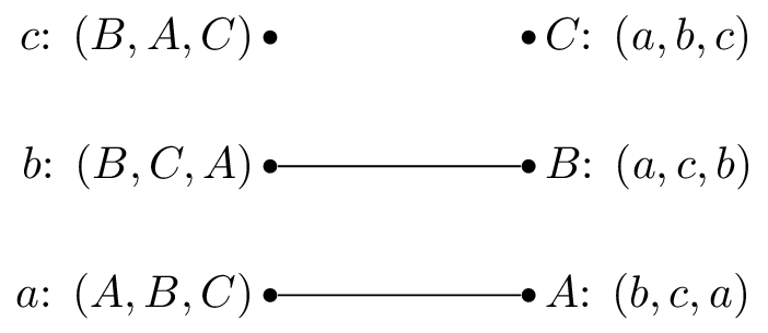
“In a population of $N$ suitors and $N$ reviewers. We allow the suitors and reviewers to rank their preferences and are now trying to match the suitors and reviewers in such a way as that every matching is stable.”

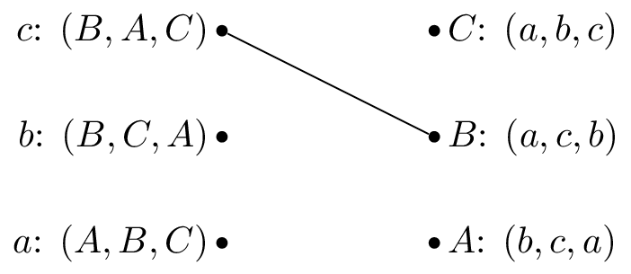
If we consider the following example with suitors: $S=\{a,b,c\}$ and reviewers: $R=\{A,B,C\}$ with preferences shown.

$A matching game.\label{L15-img01}$

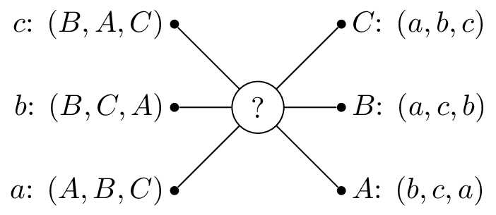
So that $A$ would prefer to be matched with $b$, then $c$ and lastly $c$. One possible matching would be is shown.

$A simple matching.\label{L15-img02}$

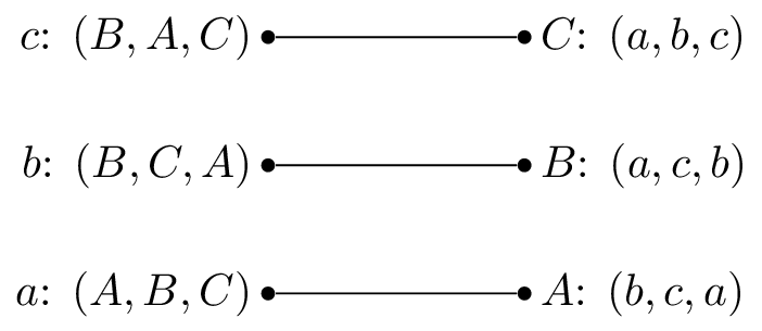
In this situation, $a$ and $b$ are getting their first choice and $c$ their second choice. However $B$ actually prefers $c$ so that matching is unstable.

Let us write down some formal definitions:

Definition of a matching game

A matching game of size $N$ is defined by two disjoint sets $S$ and $R$ or suitors and reviewers of size $N$. Associated to each element of $S$ and $R$ is a preference list:

$f:S\to R^N\text{ and }g:R\to S^N$

A matching $M$ is a any bijection between $S$ and $R$. If $s\in S$ and $r\in R$ are matched by $M$ we denote:

$M(s)=r$

Definition of a blocking pair

A pair $(s,r)$ is said to block a matching $M$ if $M(s)\ne r$ but $s$ prefers $r$ to $M(s)$ and $r$ prefers $s$ to $M^{-1}(r)$.

In our previous example $(c,B)$ blocks the proposed matching.

Definition of a stable matching

A matching $M$ with no blocking pair is said to be stable.

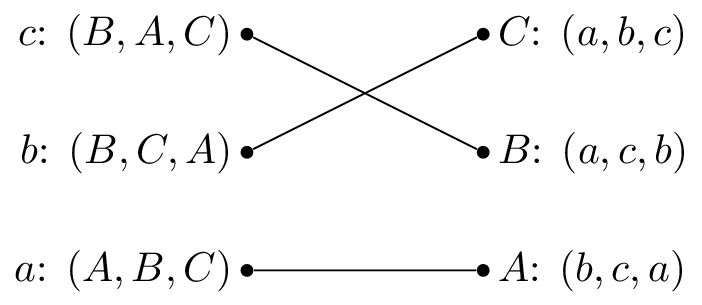
A stable matching is shown.

$A stable matching.\label{L15-img03}$

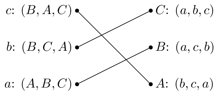
The stable matching is not unique, the matching shown is also stable:

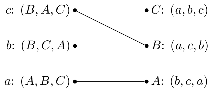
$Another stable matching.\label{L15-img04}$

The Gale-Shapley Algorithm

Here is the Gale-Shapley algorithm, which gives a stable matching for a matching game:

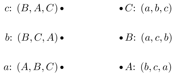
Assign every $s\in S$ and $r\in R$ to be unmatched
Pick some unmatched $s\in S$, let $r$ be the top of $s$’s preference list:
- If $r$ is unmatched set $M(s)=r$
- If $r$ is matched:
  - If $r$ prefers $s$ to $M^{-1}(r)$ then set $M(r)=s$
  - Otherwise $s$ remains unmatched and remove $r$ from $s$’s preference list.
Repeat step 2 until all $s\in S$ are matched.

Let us illustrate this algorithm with the above example.

$Base example. \label{L15-img05}$

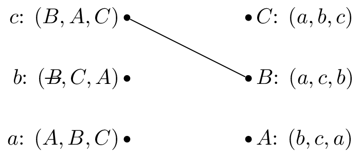
We pick $c$ and as all the reviewers are unmatched set $M(c)=B$.

$Setting $M(c)=B$. \label{L15-img06}$

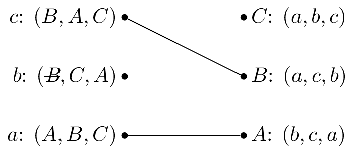
We pick $b$ and as $B$ is matched but prefers $c$ to $b$ we cross out $B$ from $b$’s preferences.

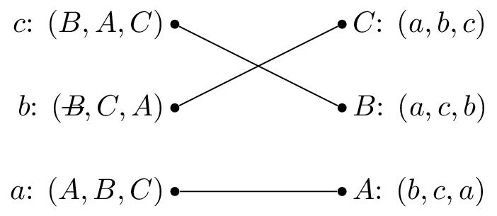
$Removing $B$ from $b$'s preference list. \label{L15-img07}$

We pick $b$ again and set $M(b)=C$.

$Setting $M(b)=C$.\label{L15-img08}$

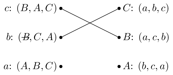
We pick $a$ and set $M(a)=A$.

$Setting $M(a)=A$. \label{L15-img04}$

Let us repeat the algorithm but pick $b$ as our first suitor.

$Base example.\label{L15-img05}$

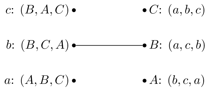
We pick $b$ and as all the reviewers are unmatched set $M(b)=B$.

$Setting $M(b)=B$. \label{L15-img09}$

We pick $a$ and as $A$ is unmatched set $M(a)=A$.

$Setting $M(a)=A$. \label{L15-img10}$

We pick $c$ and $b$ is matched but prefers $c$ to $M^{-1}(B)=b$, we set $M(c)=B$.

$Setting $M(c)=B$. \label{L15-img11}$

We pick $b$ and as $B$ is matched but prefers $c$ to $b$ we cross out $B$ from $b$’s preferences:

$Removing $B$ from $b$'s preference list. \label{L15-img12}$

We pick $b$ again and set $M(b)=C$.

$Setting $M(b)=C$. \label{L15-img13}$

Both these have given the same matching.

Theorem guaranteeing a unique matching as output of the Gale Shapley algorithm.

All possible executions of the Gale-Shapley algorithm yield the same stable matching and in this stable matching every suitor has the best possible partner in any stable matching.

Proof

Suppose that an arbitrary execution $\alpha$ of the algorithm gives $M$ and that another execution $\beta$ gives $M’$ such that $\exists$ $s\in S$ such that $s$ prefers $r’=M’(s)$ to $r=M(s)$.

Without loss of generality this implies that during $\alpha$ $r’$ must have rejected $s$. Suppose, again without loss of generality that this was the first occasion that a rejection occured during $\alpha$ and assume that this rejection occurred because $r’=M(s’)$. This implies that $s’$ has no stable match that is higher in $s’$’s preference list than $r’$ (as we have assumed that this is the first rejection).

Thus $s’$ prefers $r’$ to $M’(s’)$ so that $(s’,r’)$ blocks $M’$. Each suitor is therefore matched in $M$ with his favorite stable reviewer and since $\alpha$ was arbitrary it follows that all possible executions give the same matching.

We call a matching obtained from the Gale Shapley algorithm suitor-optimal because of the previous theorem. The next theorem shows another important property of the algorithm.

Theorem of reviewer sub optimality

In a suitor-optimal stable matching each reviewer has the worst possible matching.

Proof

Assume that the result is not true. Let $M_0$ be a suitor-optimal matching and assume that there is a stable matching $M’$ such that $\exists$ $r$ such that $r$ prefers $s=M_0^{-1}(r)$ to $s’=M’^{-1}(r)$. This implies that $(r,s)$ blocks $M’$ unless $s$ prefers $M’(s)$ to $M_0(s)$ which contradicts the fact the $s$ has no stable match that they prefer in $M_0$.

Chapter 16 - Cooperative games

Recap

In the previous chapter:

We defined matching games;
We described the Gale-Shapley algorithm;
We proved certain results regarding the Gale-Shapley algorithm.

In this Chapter we’ll take a look at another type of game.

Cooperative Games

In cooperative game theory the interest lies with understanding how coalitions form in competitive situations.

Definition of a characteristic function game

A characteristic function game G is given by a pair $(N,v)$ where $N$ is the number of players and $v:2^{[N]}\to\mathbb{R}$ is a characteristic function which maps every coalition of players to a payoff.

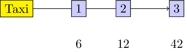
Let us consider the following game:

“3 players share a taxi. Here are the costs for each individual journey:

Player 1: 6

Player 2: 12

Player 3: 42 How much should each individual contribute?”

This is illustrated.

$A taxi journey. \label{L16-img01}$

To construct the characteristic function we first obtain the power set (ie all possible coalitions) $2^{{1,2,3}}=\{\emptyset,\{1\},\{2\},\{3\},\{1,2\},\{1,3\},\{2,3\},\Omega\}$ where $\Omega$ denotes the set of all players ($\{1,2,3\}$).

The characteristic function is given below:

$v(C)=\begin{cases} 6,&\text{if }C=\{1\}\\ 12,&\text{if }C=\{2\}\\ 42,&\text{if }C=\{3\}\\ 12,&\text{if }C=\{1,2\}\\ 42,&\text{if }C=\{1,3\}\\ 42,&\text{if }C=\{2,3\}\\ 42,&\text{if }C=\{1,2,3\}\\ \end{cases}$

Definition of a monotone characteristic function game

A characteristic function game $G=(N,v)$ is called monotone if it satisfies $v(C_2)\geq v(C_1)$ for all $C_1\subseteq C_2$.

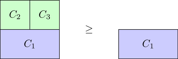
$A diagrammatic representation of monotonicity.\label{L16-img02}$

Our taxi example is monotone, however the $G=(3,v_1)$ with $v_1$ defined as:

$v_1(C)=\begin{cases} 6,&\text{if }C=\{1\}\\ 12,&\text{if }C=\{2\}\\ 42,&\text{if }C=\{3\}\\ 10,&\text{if }C=\{1,2\}\\ 42,&\text{if }C=\{1,3\}\\ 42,&\text{if }C=\{2,3\}\\ 42,&\text{if }C=\{1,2,3\}\\ \end{cases}$

is not.

Definition of a superadditive game

A characteristic function game $G=(N,v)$ is called superadditive if it satisfies $v(C_1\cup C_2)\geq v(C_1)+v(C_2).$ for all $C_1\cap C_2=\emptyset$.

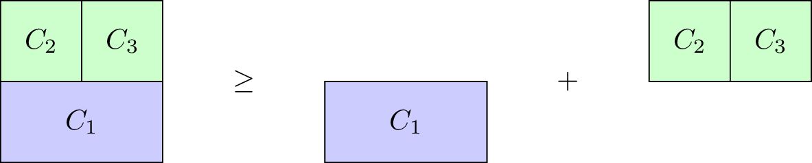
$A diagrammatic representation of superadditivity.\label{L16-img03}$

Our taxi example is not superadditive, however the $G=(3,v_2)$ with $v_2$ defined as:

$v_2(C)=\begin{cases} 6,&\text{if }C=\{1\}\\ 12,&\text{if }C=\{2\}\\ 42,&\text{if }C=\{3\}\\ 18,&\text{if }C=\{1,2\}\\ 48,&\text{if }C=\{1,3\}\\ 55,&\text{if }C=\{2,3\}\\ 80,&\text{if }C=\{1,2,3\}\\ \end{cases}$

is.

Shapley Value

When talking about a solution to a characteristic function game we imply a payoff vector $\lambda\in\mathbb{R}_{\geq 0}^{N}$ that divides the value of the grand coalition between the various players. Thus $\lambda$ must satisfy:

$\sum_{i=1}^N\lambda_i=v(\Omega)$

Thus one potential solution to our taxi example would be $\lambda=(14,14,14)$. Obviously this is not ideal for player 1 and/or 2: they actually pay more than they would have paid without sharing the taxi!

Another potential solution would be $\lambda=(6,6,30)$, however at this point sharing the taxi is of no benefit to player 1. Similarly $(0,12,30)$ would have no incentive for player 2.

To find a “fair” distribution of the grand coalition we must define what is meant by “fair”. We require four desirable properties:

Efficiency;
Null player;
Symmetry;
Additivity.

Definition of efficiency

For $G=(N,v)$ a payoff vector $\lambda$ is efficient if:

$\sum_{i=1}^N\lambda_i=v(\Omega)$

Definition of null players

For $G(N,v)$ a payoff vector possesses the null player property if $v(C\cup i)=v(C)$ for all $C\in 2^{\Omega}$ then:

$x_i=0$

Definition of symmetry

For $G(N,v)$ a payoff vector possesses the symmetry property if $v(C\cup i)=v(C\cup j)$ for all $C\in 2^{\Omega}\setminus\{i,j\}$ then:

$x_i=x_j$

Definition of additivity

For $G_1=(N,v_1)$ and $G_2=(N,v_2)$ and $G^+=(N,v^+)$ where $v^+(C)=v_1(C)+v_2(C)$ for any $C\in 2^{\Omega}$. A payoff vector possesses the additivity property if:

$x_i^{(G^+)}=x_i^{(G_1)}+x_i^{(G_2)}$

We will not prove in this course but in fact there is a single payoff vector that satisfies these four properties. To define it we need two last definitions.

Definition of predecessors

If we consider any permutation $\pi$ of $[N]$ then we denote by $S_\pi(i)$ the set of predecessors of $i$ in $\pi$:

$S_\pi(i)=\{j\in[N]\;|\;\pi(j)<\pi(i)\}$

For example for $\pi=(1,3,4,2)$ we have $S_\pi(4)=\{1,3\}$.

Definition of marginal contribution

If we consider any permutation $\pi$ of $[N]$ then the marginal contribution of player $i$ with respect to $\pi$ is given by:

$\Delta_\pi^G(i)=v(S_{\pi}(i)\cup i)-v(S_{\pi}(i))$

We can now define the Shapley value of any game $G=(N,v)$.

Definition of the Shapley value

Given $G=(N,v)$ the Shapley value of player $i$ is denoted by $\phi_i(G)$ and given by:

$\phi_i(G)=\frac{1}{N!}\sum_{\pi\in\Pi_n}\Delta_\pi^G(i)$

As an example here is the Shapley value calculation for our taxi sharing game:

For $\pi=(1,2,3)$:

$\begin{aligned} \Delta_{\pi}^G(1)&=6\\ \Delta_{\pi}^G(2)&=6\\ \Delta_{\pi}^G(3)&=30\\ \end{aligned}$

For $\pi=(1,3,2)$:

$\begin{aligned} \Delta_{\pi}^G(1)&=6\\ \Delta_{\pi}^G(2)&=0\\ \Delta_{\pi}^G(3)&=36\\ \end{aligned}$

For $\pi=(2,1,3)$:

$\begin{aligned} \Delta_{\pi}^G(1)&=0\\ \Delta_{\pi}^G(2)&=12\\ \Delta_{\pi}^G(3)&=30\\ \end{aligned}$

For $\pi=(2,3,1)$:

$\begin{aligned} \Delta_{\pi}^G(1)&=0\\ \Delta_{\pi}^G(2)&=12\\ \Delta_{\pi}^G(3)&=30\\ \end{aligned}$

For $\pi=(3,1,2)$:

$\begin{aligned} \Delta_{\pi}^G(1)&=0\\ \Delta_{\pi}^G(2)&=0\\ \Delta_{\pi}^G(3)&=42\\ \end{aligned}$

For $\pi=(3,2,1)$:

$\begin{aligned} \Delta_{\pi}^G(1)&=0\\ \Delta_{\pi}^G(2)&=0\\ \Delta_{\pi}^G(3)&=42\\ \end{aligned}$

Using this we obtain:

$\phi(G)=(2,5,35)$

Thus the fair way of sharing the taxi fare is for player 1 to pay 2, player 2 to pay 5 and player 3 to pay 35.

Chapter 17 - Routing Games

Recap

In the previous chapter:

We defined characteristic function games;
We defined the Shapley value.

In this chapter we’ll take a look at another type of game that allows us to model congestion.

Routing games

Game theory can be used to model congestion in a variety of settings:

Road traffic;
Data traffic;
Patient flow in healthcare;
Strategies in basketball.

The type of game used is referred to as a routing game.

Definition of a routing game

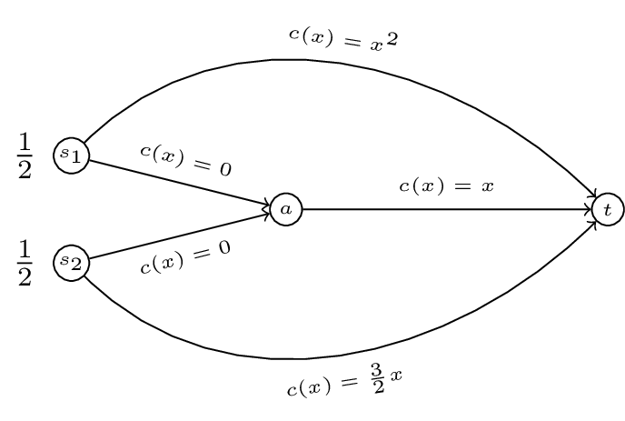
A routing game $(G,r,c)$ is defined on a graph $G=(V,E)$ with a defined set of sources $s_i$ and sinks $t_i$. Each source-sink pair corresponds to a set of traffic (also called a commodity) $r_i$ that must travel along the edges of $G$ from $s_i$ to $t_i$. Every edge $e$ of $G$ has associated to it a nonnegative, continuous and nondecreasing cost function (also called latency function) $c_e$.

An example of such a game is given.

$A simple di-graph.\label{L17-img01}$

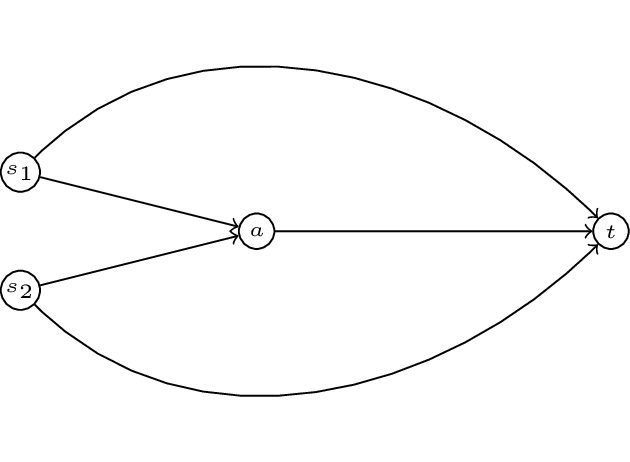
In this game we have two commodoties with two sources: $s_1$ and $s_2$ and a single sink $t$. To complete our definition of a routing game we require a quantity of traffic, let $r=(1/2,1/2)$. We also require a set of cost functions $c$. Let:

$\begin{aligned} c_{s_1a}&=0\\ c_{s_2a}&=0\\ c_{s_1t}&=x^2\\ c_{s_2t}&=\frac{3x}{2}\\ c_{at}&=x\\ \end{aligned}$

We represent all this diagrammatically.

$A routing game. \label{L17-img02}$

Definition of the set of paths

For any given $(G,r,c)$ we denote by $\mathcal{P}_i$ the set of paths available to commodity $i$.

For our example we have:

$\mathcal{P}_1=\{s_1at,s_1t\}$

and

$\mathcal{P}_2=\{s_2at,s_2t\}$

We denote the set of all possible paths by $\mathcal{P}=\bigcup_{i}\mathcal{P}_i$.

Definition of a feasible flow

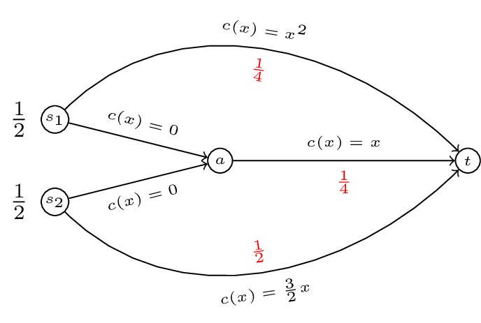
On a routing game we define a flow $f$ as a vector representing the quantity of traffic along the various paths, $f$ is a vector index by $\mathcal{P}$. Furthermore we call $f$ feasible if:

$\sum_{P\in\mathcal{P}_i}f_P=r_i$

In our running example $f=(1/4,1/4,0,1/2)$ is a feasible flow.

$A feasible flow.\label{L17-img03}$

To go further we need to try and measure how good a flow is.

Optimal flow

Definition of the cost function

For any routing game $(G,r,c)$ we define a cost function $C(f)$:

$C(f)=\sum_{P\in\mathcal{P}}c_P(f_P)f_P$

Where $c_P$ denotes the cost function of a particular path $P$: $c_P(x)=\sum_{e\in P}c_e(x)$. Note that any flow $f$ induces a flow on edges:

$f_e=\sum_{P\in\mathcal{P}\text{ if }e\in P}f_P$

So we can re-write the cost function as:

$C(f)=\sum_{e\in E}c_e(f_e)f_e$

Thus for our running example if we take a general $f=(\alpha,1/2-\alpha,1/2-\beta,\beta)$ as shown.

$A generic flow.\label{L17-img04}$

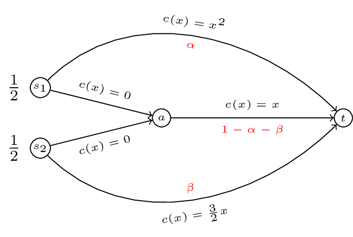
The cost of $f(\alpha,1/2-\alpha,1/2-\beta,\beta)$ is given by:

$\begin{aligned} C(f)&=\alpha^2\times\alpha+3/2\beta\times\beta+(1-\alpha-\beta)\times(1-\alpha-\beta)\\ &=\alpha^3+3/2\beta^2+\alpha^2 + 2\alpha\beta + \beta^2 - 2\alpha - 2\beta + 1 \end{aligned}$

Definition of an optimal flow

For a routing game $(G,r,c)$ we define the optimal flow $f^*$ as the solution to the following optimisation problem:

Minimise $\sum_{e\in E}c_e(f_e)f_e$:

Subject to:

$\begin{aligned} \sum_{P\in\mathcal{P}_i}f_P&=r_i&&\text{for all }i\\ f_e&=\sum_{P\in\mathcal{P}\text{ if }e\in P}f_P&&\text{ for all }e\in E\\ f_P&\geq 0 \end{aligned}$

In our example this corresponds to minimising $C(\alpha,\beta)=\alpha^3+3/2\beta^2+\alpha^2 + 2\alpha\beta + \beta^2 - 2\alpha - 2\beta + 1$ such that $0\leq\alpha\leq 1/2$ and $0\leq\beta\leq1/2$.

A plot of $C(\alpha,\beta)$ is shown.

$$C(\alpha,\beta)$.\label{L17-plot01}$

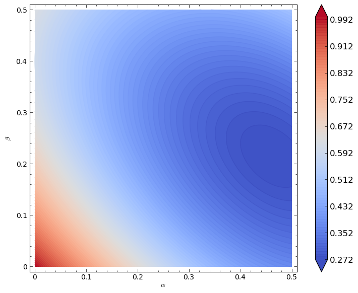
It looks like the minimal point is somewhere near higher values of $\alpha$ and $\beta$. Let us carry out our optimisation properly:

If define the Lagrangian:

$L(\alpha,\beta,\lambda_1,\lambda_2,\lambda_3,\lambda_4)=C(\alpha,\beta)-\lambda_1\alpha-\lambda_2(\alpha-1/2)-\lambda_3\beta-\lambda_4\beta$

This will work but creates a large number of variables (so things will get messy quickly). Instead let us realise that the minima will either be in the interior of our region or on the boundary of our region.

If it is on the interior of the region then we will have:

$\frac{\partial C}{\partial \alpha}=3\alpha^2-2(1-\alpha-\beta)=0$ and $\frac{\partial C}{\partial \beta}=3\beta-2(1-\alpha-\beta)=0$

which gives:

$\beta=\frac{2(1-\alpha)}{5}$

Substituting this in to the first equation gives:

$3\alpha^2-\frac{6}{5}(1-\alpha)=0$

which has solution (in our region):

$\alpha_1=\frac{\sqrt{11}-1}{5}\approx 0.4633$ giving: $\beta_1=0.2147$

Firstly $(\alpha_1,\beta_1)$ is located in the required region. Secondly it is straightforward to verify that this is a local minima (by checking the second derivatives).

We have $C(\alpha_1,\beta_1)=\frac{3}{125} \left(\sqrt{11} - 6\right)^{2} + \frac{1}{125}\left(\sqrt{11} - 1\right)^{3}\approx .2723$.

To verify that this is an optimal flow we need to verify that it is less than all values on the boundaries. We first calculate the values on the extremal points of our boundary:

$C(0,0)=1$
$C(0,1/2)=5/8=.625$
$C(1/2,0)=3/8=.375$
$C(1/2,1/2)=1/2=.5$

We now check that there are no local optima on the boundary:

Consider $C(\alpha,0)=\alpha^3+\alpha^2-2\alpha+1$ equating the derivative to 0 gives: $3\alpha^2+2\alpha-2=0$ which has solution $\alpha=\frac{-1\pm\sqrt{7}}{3}$. We have $C(\frac{-1+\sqrt{7}}{3},0)\approx.3689$.
Consider $C(\alpha,1/2)=\alpha^3+\alpha^2-\alpha+5/8$ equating the derivative to 0 gives: $3\alpha^2+2\alpha-1=0$ which has solution $\alpha=1/3$ and $\alpha=1$. We have $C(1/3,1/2)\approx.4398$
When considering $C(0,\beta)$ we know that the local optima is at $\beta=\frac{2}{5}$. We have $C(0,2/5)=.6$.
Similarly when considering $C(1/2,\beta)$ we know that the local optima is at $\beta=\frac{2(1-1/2)}{5}$. We have $C(1/2,1/5)=.275$.

Thus $f^*\approx(.4633,0.2147)$.

Nash flows

If we take a closer look at $f^*$ in our example, we see that traffic from the first commodity travels across two paths: $P_1=s_1t$ and $P_2=s_1at$. The cost along the first path is given by:

$C_{P_1}(f^*)=.4633^2\approx.2146$

The cost along the second path is given by:

$C_{P_2}(f^*)=(1-.4633-.2147)\approx .3220$

Thus traffic going along the second path is experiencing a higher cost. If this flow represented commuters on their way to work in the morning users of the second path would deviate to use the first. This leads to the definition of a Nash flow.

Definition of a Nash flow

For a routing game $(G,r,c)$ a flow $\tilde f$ is called a Nash flow if and only if for every commodity $i$ and any two paths $P_1,P_2\in\mathcal{P}_i$ such that $f_{P_1}>0$ then:

$c_{P_1}(f)\leq c_{P_2}(f)$

In other words a Nash flow ensures that all used paths have minimal costs.

If we consider our example and assume that both commodities use all paths available to them:

$\begin{aligned} \alpha^2&=1-\alpha-\beta\\ \frac{3\beta}{2}&=1-\alpha-\beta \end{aligned}$

Solving this gives: $\beta=\frac{2}{5}(1-\alpha)$ $\Rightarrow$ $x^{2} + \frac{3}{5} \, x - \frac{3}{5}$ this gives $\alpha\approx .5307$ which is not in our region. Let us assume that $\alpha=1/2$ (i.e. commodity 1 does not use $P_2$). Assuming that the second commodity uses both available paths we have:

$\frac{3}{2}\beta=\frac{1}{2}-\beta\Rightarrow\beta=\frac{1}{5}$

We can check that all paths have minimal cost.

Thus we have $\tilde f=(1/2,1/5)$ which gives a cost of $C(\tilde f)=11/40$ (higher than the optimal cost!).

What if we had assumed that $\beta=1/2$?

This would have given $\alpha^2=1/2-\alpha$ which has solution $\alpha\approx .3660$. The cost of the path $s_2at$ is then $.134$ however the cost of the path $s_2t$ is $.75$ thus the second commodity should deviate. We can carry out these same checks with all other possibilities to verify that $\tilde f=(1/2,1/5)$.

Chapter 18 - Connection between optimal and Nash flows

Recap

In the previous chapter:

We defined routing games;
We defined and calculated optimal flows;
We defined and calculated Nash flows.

In this Chapter we’ll look at the connection between Optimal and Nash flows.

Potential function

Definition of a potential flow

Given a routing game $(G,r,c)$ we define the potential function of a flow as:

$\Phi(f)=\sum_{e\in E}\int_0^{f_e}c_e(x)dx$

$A routing game.\label{L17-img04}$

Thus for the routing game shown we have:

$\Phi((\alpha,\beta))=\frac{\alpha^3}{3}+\frac{3\beta^2}{4}+\frac{(1-\alpha-\beta)^2}{2}$

A plot of $\Phi(\alpha,\beta)$ is shown.

$$\Phi(\alpha,\beta)$.\label{L18-plot01}$

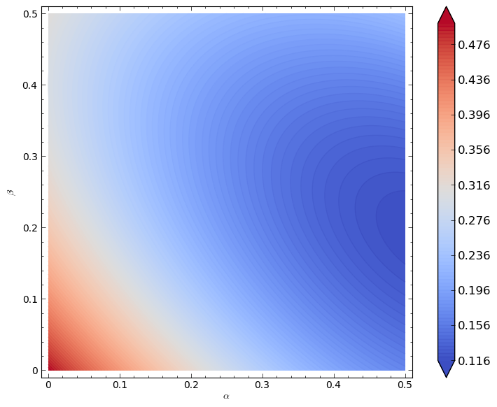
We can verify analytically (as before) that the minimum of this function is given by $(\alpha,\beta)=(1/2,1/5)$. This leads to the following powerful result.

Theorem connecting the Nash flow to the optimal flow

A feasible flow $\tilde f$ is a Nash flow for the routing game $(G,r,c)$ if and only if it is a minima for $\Phi(f)$.

This is a very powerful result that allows us to obtain Nash flows using minimisation techniques.

It also points towards a connection between Nash flows and optimal flows.

Marginal costs

Definition of marginal cost

If $c$ is a differentiable cost function then we define the marginal cost function $c^*$ as:

$c^*=\frac{d}{dx}(xc(x)$

For our running example we have the marginal cost functions given.

$$(G,r,c)$.\label{L18-img01}$

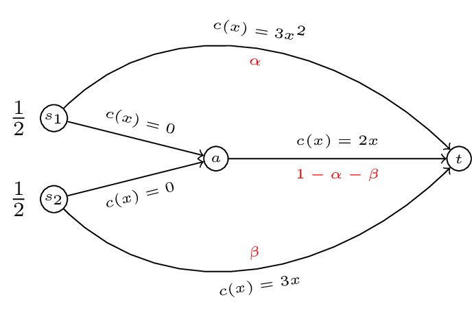
We now state our last theorem of the course:

Theorem connecting optimal flows to Nash flows

A feasible flow $f^*$ is an optimal flow for $(G,r,c)$ if and only if $f^*$ is a Nash flow for $(G,r,c^*)$.

Using this we can compute the optimal flow for our original game by computing the Nash flow for our modified game.

If we assume that both players use both paths then we have:

$\begin{aligned} 3\alpha^2&=2(1-\alpha-\beta)\\ 3\beta&=2(1-\alpha-\beta) \end{aligned}$

This gives $\beta=\frac{2}{5}(1-\alpha)$ implying $3\alpha^2=\frac{6}{5}(1-\alpha)$ which gives (as before) $f^* \approx(.4633,0.2147)$.

We will finish the course by looking at an interesting example that occurs in routing game theory.

Braess’s Paradox

Consider the routing game shown.

$A simple routing game.\ref{L18-img02}$

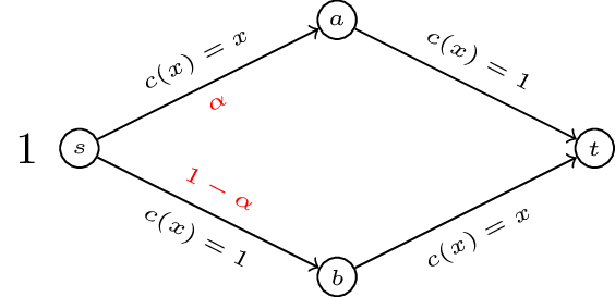
If we write down the potential function $\Phi(\alpha)=\alpha^2/2+(1-\alpha)^2/2+(1-\alpha)+\alpha=\alpha^2 -\alpha + 3/2$. The flow $\tilde f=1/2$ minimises the potential function and so is a Nash flow. In fact for this example we have $\tilde f=f^*$ and $C(\tilde f)=C(f^*)=3/2$.

If we modify the network by adding capacity to our network with another edge of zero cost.

$Brass's Paradox. \label{L18-img03}$

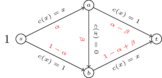
We can compute the potential function and optimise but we can quickly verify that $\tilde f=(\alpha,\beta)=(1,1)$ is a Nash flow by comparing with other potential paths. Thus we have $C(\tilde f)=2$. By adding an edge to our network with a very “cheap” latency cost the situation has been made worse!

Programming

There are various areas of Game theory that are suited to computer programming.

The two areas that naturally sit in this course are:

The computation of equilibria;
The study of the Iterated Prisoner’s Dilemma

A quick refresher of using Python

Note that this refresher uses Python 3 and will also go over the use of external libraries.

I recommend using Anaconda as a distribution of Python. Go to https://www.continuum.io/downloads and follow the instructions there.
Basics of Python using Jupyter notebooks.
- Code example
- Video walk through
External libraries.
- Code example
- Video walk through

Computation of equilibria

To compute equilibria there are 3 pieces of software available to you:

Cloud.sagemath (using Sage). Documentation: doc.sagemath.org/html/en/reference/game_theory/index.html
NashPy (a standalone Python library).
- Code example
- Video walk through
Gambit (a piece of software with a Python interface): gambit.sourceforge.net/.

Studying the Iterated Prisoners’ Dilemma

The main library used for the study of the Iterated Prisoners’ Dilemma is the Axelrod Python library.

Documentation

All chapters

{% for page in site.pages %} {% if page.categories contains ‘content’ %} —

{% endif %} {% endfor %}

Introduction

2/3rds of the average game

Extensive Form Games

Definition of an Extensive form game

Example: Battle of the sexes

Information sets

Definition of an Information set

Recap

Normal form games

Definition of a normal form game

Some examples

The battle of the sexes

Prisoners’ Dilemma

Hawk-Dove

Pigs

Matching pennies

Mixed Strategies

Definition of a mixed strategy

Matching pennies revisited.

Example

Recap

Dominant strategies

Definition of an incomplete strategy profile

Definition of a strictly dominated strategy

Definition of a weakly dominated strategy

Common knowledge of rationality

Example

Example

Not all games can be solved using dominance

Recap

Best response functions

Definition of a best response

Best responses against mixed strategies

Connection between best responses and dominance

Definition of the undominated strategy set

Definition of the best responses strategy set

Theorem of equality in 2 player games

Theorem of inclusion in \(N\) player games

Recap

Nash equilibria

Definition of Nash equilibria

Example

Duopoly game

Recap

Recall of expected utility calculation

Obtaining equilibria

Equality of payoffs theorem

Definition of the support of a strategy

Theorem of equality of payoffs

Proof

Example

Nash’s Theorem

Recap

Extensive form games

Backwards induction

Definition of sequential rationality

Definition of backward induction

Example

Theorem of existence of Nash equilibrium in games of perfect information.

Proof

Stackelberg game

Recap

Connection between extensive and normal form games

Subgames

Definition of a subgame

Subgame perfect equilibria

Definition of subgame perfect equilibrium

Recap

Repeated games

Definition of a repeated game

Definition of a strategy in a repeated game

Subgame perfect Nash equilibrium in repeated games

Theorem of a sequence of stage Nash profiles

Proof

Example

Reputation in repeated games

Recap

Discounting

Conditions for cooperation in Prisoner’s Dilemmas

Folk theorem