Chapter 14 - Stochastic games

Recap

In the previous chapter:

We considered games of incomplete information;
Discussed some basic utility theory;
Considered the principal agent game.

In this chapter we will take a look at a more general type of random game.

Stochastic games

Definition of a stochastic game

A stochastic game is defined by:

X a set of states with a stage game defined for each state;
A set of strategies $S_i(x)$ for each player for each state $x\in X$;
A set of rewards dependant on the state and the actions of the other players: $u_i(x,s_1,s_2)$;
A set of probabilities of transitioning to a future state: $\pi(x’|x,s_1,s_2)$;
Each stage game is played at a set of discrete times $t$.

We will make some simplifying assumptions in this course:

The length of the game is not known (infinite horizon) - so we use discounting;
The rewards and transition probabilities are not dependent;
We will only consider strategies called Markov strategies.

Definition of a Markov strategy

A strategy is call a Markov strategy if the behaviour dictated is not time dependent.

Example

Consider the following game with $X=\{x,y\}$:

$S_1(x)=\{a,b\}$ and $S_2(x)=\{c,d\}$;
$S_1(y)=\{e\}$ and $S_2(x)=\{f\}$;

We have the stage game corresponding to state $x$:

$\begin{pmatrix} (8,4)&(5,3)\\ (1,5)&(2,6) \end{pmatrix}$

The stage game corresponding to state $y$:

$\begin{pmatrix} (0,0)\\ \end{pmatrix}$

The transition probabilities corresponding to state $x$:

$\begin{pmatrix} (.5,.5)&(1,0)\\ (1,0)&(1,0) \end{pmatrix}$

The transition probabilities corresponding to state $y$:

$\begin{pmatrix} (0,1)\\ \end{pmatrix}$

A concise way of representing all this is shown.

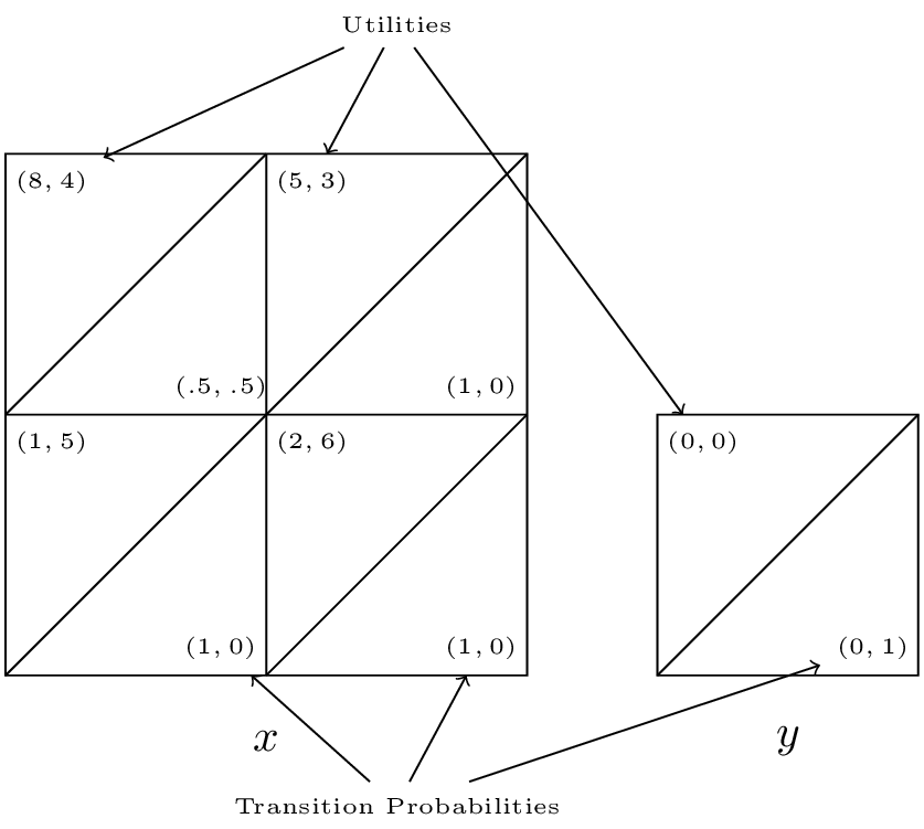
$A simple stochastic game.\label{L14-img01}$

We see that the Nash equilibrium for the stage game corresponding to $x$ is $(a, c)$ however as soon as the players play that strategy profile they will potentially go to state $y$ which is an absorbing state at which players gain no further utility.

To calculate utilities for players in infinite horizon stochastic games we use a discount rate. Thus without loss of generality if the game is in state $x$ and we assume that both players are playing $\sigma^*_i$ then player 1 would be attempting to maximise future payoffs:

$U_1(r,c)=\left(u_1(x,r,c)+\delta\sum_{x'\in X}\pi(x'|x,r,c)U_1^*(x')\right)$

where $U_1^*$ denotes the expected utility to player 1 when both players are playing the Nash strategy profile.

Thus a Nash equilibrium satisfies:

$U_1^*(x)=\max_{r\in S_1(x)}(u_i(x,r,c^* )+\delta\sum_{x'\in X}\pi(x'|x,r,c^*)U_1^*(x'))$ $U_2^*(x)=\max_{c\in S_2(x)}(u_i(x,r^*,c)+\delta\sum_{x'\in X}\pi(x'|x,r^*,c)U_2^*(x'))$

Solving these equations is not straightforward. We will take a look at one approach by solving the example we have above.

Finding equilibria in stochastic games

Let us find a Nash equilibrium for the game considered above with $\delta=2/3$.

State $y$ gives no value to either player so we only need to consider state $x$. Let the future gains to player 1 in state $x$ be $v$, and the future gains to player 2 in state $x$ be $u$. Thus the players are facing the following game:

$\begin{pmatrix} (8+\frac{1}{3}v,4+\frac{1}{3}u)&(5+\frac{2}{3}v,3+\frac{2}{3}u)\\ (1+\frac{2}{3}v,5+\frac{2}{3}u)&(2+\frac{2}{3}v,6+\frac{2}{3}u) \end{pmatrix}$

We consider each strategy pair and state the condition for Nash equilibrium:

$(a,c)$: $v\leq 21$ and $u\leq 3$.
$(a,d)$: $u\geq3$.
$(b,c)$: $v\geq 21$ and $5\geq 6$.
$(b,d)$: $5\leq2$.

Now consider the implications of each of those profiles being an equilibrium:

$8+v/3=v$ $\Rightarrow$ $v=12$ and $4+u/3=u$ $\Rightarrow$ $u=6$ which contradicts the corresponding inequality.
$3+2u/3=u$ $\Rightarrow$ $u=9$.
The second inequality cannot hold.
The inequality cannot hold.

Thus the unique Markov strategy Nash equilibria is $(a,d)$ which is not the stage Nash equilibria!