Playing against a mixed strategy in class

This post if very late but I have been very busy with some really exciting things. I will describe some of the data gathered in class when we played against a random strategy played by a computer. I have recently helped organise a conference in Namibia teaching Python. It was a tremendous experience and I will write a post about that soon.

We played against a modified version of matching pennies which we have used quite a few times:

$\begin{pmatrix} (2,-2) & (-2,2)\\ (-1,1) & (1,-1) \end{pmatrix}$

I wrote a sage interact that allows for a quick visualisation of a random sample from a mixed strategy. You can find the code for that at the blog post I wrote last year. You can also find a python script with all the data from this year here.

I handed out sheets of papers on which students would input their preferred strategies (‘H’ or ‘T’) whilst I sampled randomly from 3 different mixed strategies:

$\sigma_1 = (.2, .8)$
$\sigma_1 = (.9, .1)$
$\sigma_1 = (1/3, 2/3$

Based on the class notation that implies that the computer was the row player and the students the column player. The sampled strategies were (we played 6 rounds for each mixed strategy):

TTTTTH
HHHHHH
HTTTHH

Round 1

This mixed strategy (recall $\sigma_1=(.2,.8)$) implies that the computer will be mainly playing T (the second strategy equivalent to the second row), and so based on the bi-matrix it is in the students interest to play H. Here is a plot of the mixed strategy played by all the students:

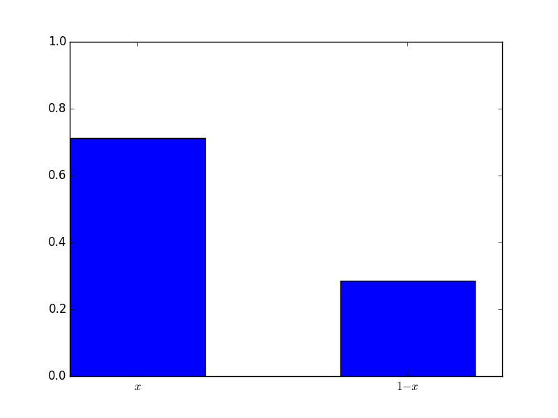
The mixed strategy played was $\sigma_2=(.71,.29)$. Note that in fact in this particular instance that actual best response is to play $\sigma_2=(1,0)$. This will indeed maximise the expected value of:

$u_2(\sigma_1, (x, 1-x)) = -2 \times .2 \times x + .8 \times x + 2 \times .2 \times (1-x) - .8 \times (1-x) = .8x-.4$

Indeed: the above is an increasing linear function in $x$ so the highest value is obtained when $x=1$.

The mean score for this round by everyone was: 2.09. The theoretical mean score (when playing the best response for six consecutive games is): $6(-.2\times 2+.8)=2.4$, so everybody was not too far off.

Here is a distribution of the scores:

We see that there were very few losers in this round, however no students obtained the best possible score: 7.

Round 2

Here the mixed strategy is $\sigma_1=(.9,.1)$, implying that students should play T more often than H. Here is a plot of the mixed strategy played by all the students:

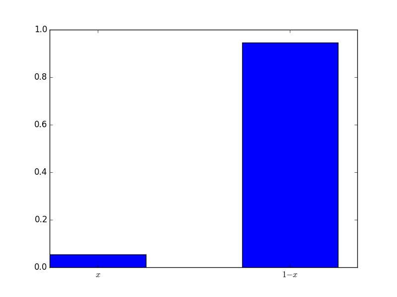
The mixed strategy played was $\sigma_2=(.05,.95)$. Similarly to before this is close to the actual best response which is $(0,1)$ (due to the expected utility now being a decreasing linear function in $x$.

The mean score for this round by everyone was: 10.69 The theoretical mean score (when playing the best response for six consecutive games is): $6(.9\times 2-.1)=10.2$, which is less than the score obtained by the class (mainly because the random sampler did not actually pick T at any point).

Here is a distribution of the scores:

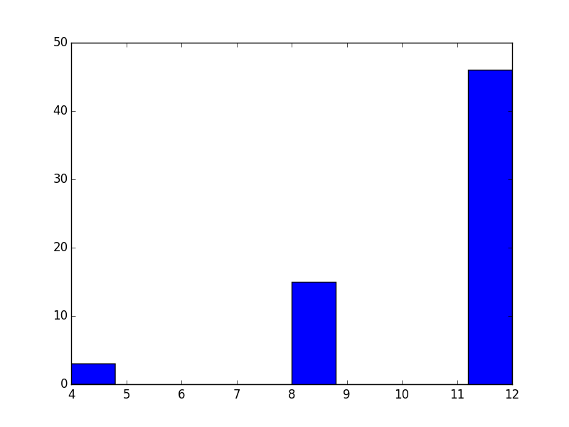
No one lost on this round and a fair few maxed out at 12.

Round 3

Here is where things get interesting. The mixed strategy played by the computer is here $\sigma_1=(1/3,2/3)$, it is not now obvious which strategy is worth going for!

Here is the distribution played:

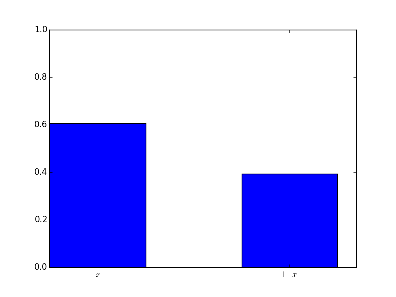
The mixed strategy is $\sigma_2=(.61,.39)$ and the mean score was -.3. Here is what the distribution looked like:

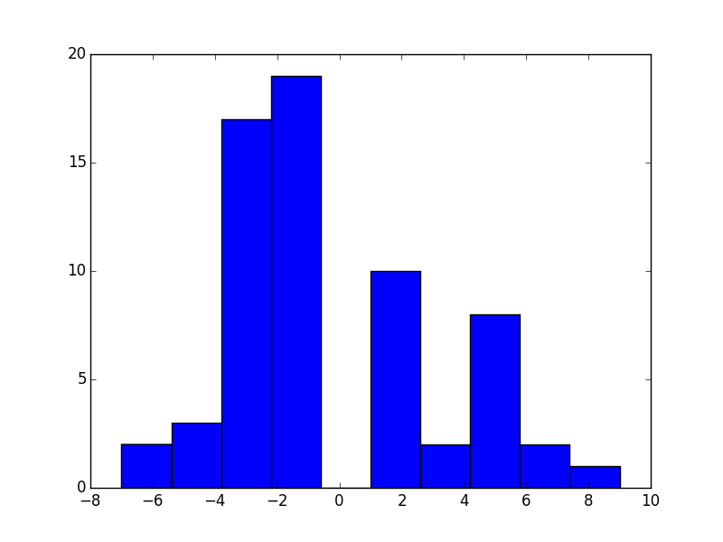
It looks like we have a few more losers than winners but not by much. In fact I would suggest (because I know the theory covered in Chapter 5 of my class) that the students were in fact indifferent against this $\sigma_1$. Indeed:

$u_2(\sigma_1,(1,0))=\frac{-2}{3}+\frac{2}{3}=0$

and

$u_2(\sigma_1,(0,1))=\frac{2}{3}+\frac{-2}{3}=0$

In fact, this particular $\sigma_1$ ensures that the expected result for the students is not influenced by what they actually do:

$u_2(\sigma_1,(x,1-x))=\frac{1}{3}(-2x+2-2x)+\frac{2}{3}(x-1+x)=\frac{2}{3}(1-2x)\frac{2}{3}(2x-1)=0$

What strategy could the students have played to ensure the same situation for the computer’s strategy? At the moment, the mixed strategy $\sigma_2=(.61,.39)$ has expected utility for player 1 (the computer):

$u_1((x,1-x), \sigma_2)=.61(2x-1+x)+.39(-2x+1-x)=0.66x - 0.22$

As this is an increasing function in $x$ we see that the computer should in fact change $\sigma_1$ to be $(1,0)$.

Thus if the original $\sigma_1$ of this round is being played, so that the choice of $\sigma_2$ does in fact not have an effect, students might as well play a strategy that ensures that the computer has no incentive to deviate (ie we are at a Nash equilibrium).

This can be calculated by solved the following linear equation:

$u_1((1,0),(x,1-x))=u_1((0,1),(x,1-x))$

which corresponds to:

$2x-2+2x=-x+1-x \Rightarrow 4x-2=1-2x$

which gives a strategy at which the computer has no incentive to deviated: $(1/2,1/2)$. Thus at $\sigma_1=(1/3,2/3)$ and $\sigma_2=(1/2,1/2)$ no players have an incentive to move: we are at a Nash equilibrium. This actually brings us back to another post I’ve written this term so please do go take a look at this post which involved students playing against each other and comparing to the Nash equilibrium.