Visualising Markov Chains with NetworkX
I’ve written quite a few blog posts about Markov chains (it occupies a central role in quite a lot of my research). In general I visualise 1 or 2 dimensional chains using Tikz (the LaTeX package) sometimes scripting the drawing of these using Python but in this post I’ll describe how to use the awesome networkx package to represent the chains.
For all of this we’re going to need the following three imports:
from __future__ import division  # Only for how I'm writing the transition matrix
import networkx as nx  # For the magic
import matplotlib.pyplot as plt  # For plotting
Let’s consider the Markov Chain I describe in this post about waiting times in a tandem queue. You can see an image of it (drawn in Tikz) below:
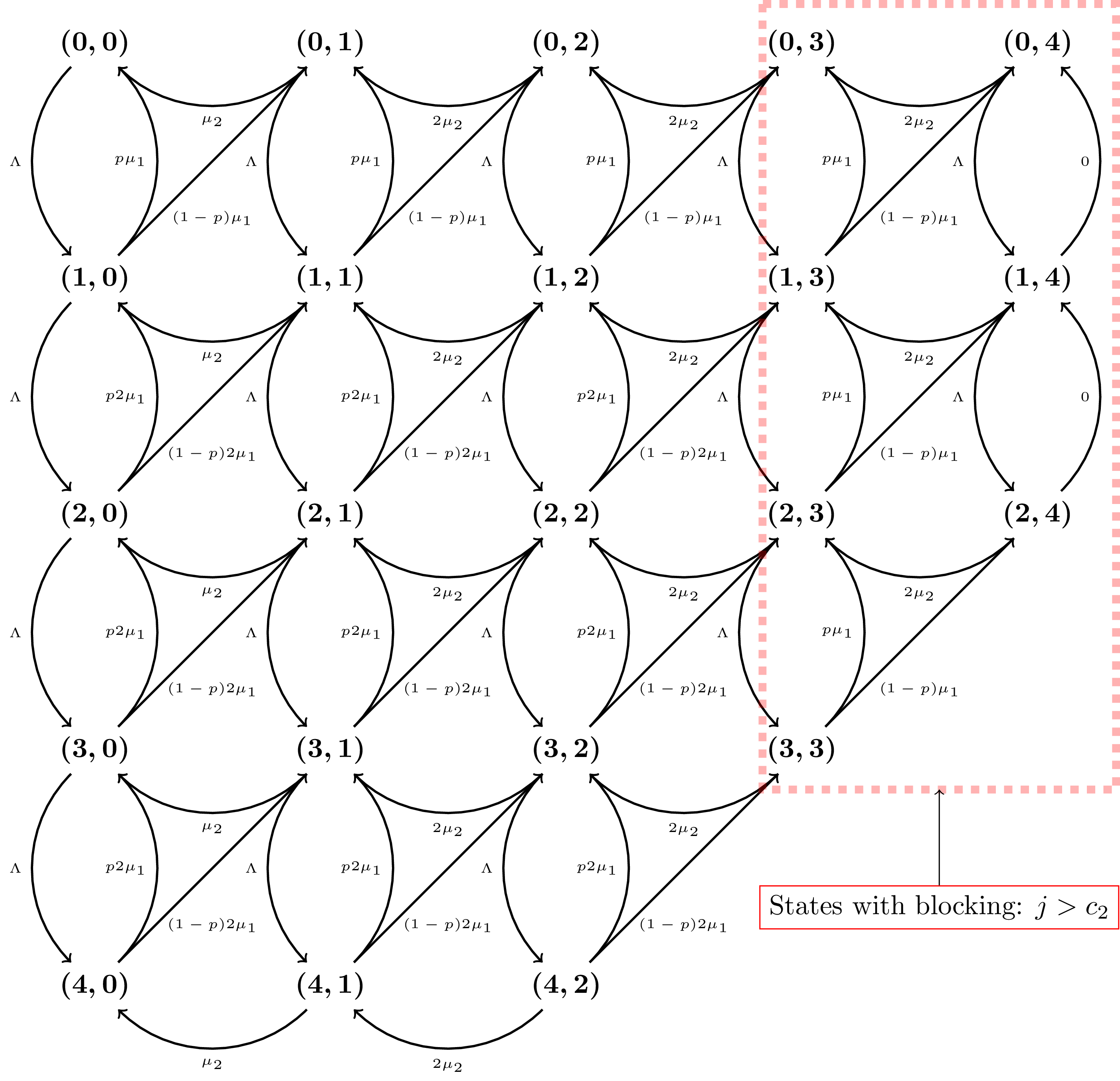
As is described in that post, we’re dealing with a two dimensional chain and without going in to the details, the states are given by:
states = [(0, 0),
          (1, 0),
          (2, 0),
          (3, 0),
          (4, 0),
          (0, 1),
          (1, 1),
          (2, 1),
          (3, 1),
          (4, 1),
          (0, 2),
          (1, 2),
          (2, 2),
          (3, 2),
          (4, 2),
          (0, 3),
          (1, 3),
          (2, 3),
          (3, 3),
          (0, 4),
          (1, 4),
          (2, 4)]
and the transition matrix \(Q\) by:
Q = [[-5, 5, 0, 0, 0, 0, 0, 0, 0, 0, 0, 0, 0, 0, 0, 0, 0, 0, 0, 0, 0, 0],
     [1/2, -6, 5, 0, 0, 1/2, 0, 0, 0, 0, 0, 0, 0, 0, 0, 0, 0, 0, 0, 0, 0, 0],
     [0, 1, -7, 5, 0, 0, 1, 0, 0, 0, 0, 0, 0, 0, 0, 0, 0, 0, 0, 0, 0, 0],
     [0, 0, 1, -7, 5, 0, 0, 1, 0, 0, 0, 0, 0, 0, 0, 0, 0, 0, 0, 0, 0, 0],
     [0, 0, 0, 1, -2, 0, 0, 0, 1, 0, 0, 0, 0, 0, 0, 0, 0, 0, 0, 0, 0, 0],
     [1/5, 0, 0, 0, 0, -26/5, 5, 0, 0, 0, 0, 0, 0, 0, 0, 0, 0, 0, 0, 0, 0, 0],
     [0, 1/5, 0, 0, 0, 1/2, -31/5, 5, 0, 0, 1/2, 0, 0, 0, 0, 0, 0, 0, 0, 0, 0, 0],
     [0, 0, 1/5, 0, 0, 0, 1, -36/5, 5, 0, 0, 1, 0, 0, 0, 0, 0, 0, 0, 0, 0, 0],
     [0, 0, 0, 1/5, 0, 0, 0, 1, -36/5, 5, 0, 0, 1, 0, 0, 0, 0, 0, 0, 0, 0, 0],
     [0, 0, 0, 0, 1/5, 0, 0, 0, 1, -11/5, 0, 0, 0, 1, 0, 0, 0, 0, 0, 0, 0, 0],
     [0, 0, 0, 0, 0, 2/5, 0, 0, 0, 0, -27/5, 5, 0, 0, 0, 0, 0, 0, 0, 0, 0, 0],
     [0, 0, 0, 0, 0, 0, 2/5, 0, 0, 0, 1/2, -32/5, 5, 0, 0, 1/2, 0, 0, 0, 0, 0, 0],
     [0, 0, 0, 0, 0, 0, 0, 2/5, 0, 0, 0, 1, -37/5, 5, 0, 0, 1, 0, 0, 0, 0, 0],
     [0, 0, 0, 0, 0, 0, 0, 0, 2/5, 0, 0, 0, 1, -37/5, 5, 0, 0, 1, 0, 0, 0, 0],
     [0, 0, 0, 0, 0, 0, 0, 0, 0, 2/5, 0, 0, 0, 1, -12/5, 0, 0, 0, 1, 0, 0, 0],
     [0, 0, 0, 0, 0, 0, 0, 0, 0, 0, 2/5, 0, 0, 0, 0, -27/5, 5, 0, 0, 0, 0, 0],
     [0, 0, 0, 0, 0, 0, 0, 0, 0, 0, 0, 2/5, 0, 0, 0, 1/2, -32/5, 5, 0, 1/2, 0, 0],
     [0, 0, 0, 0, 0, 0, 0, 0, 0, 0, 0, 0, 2/5, 0, 0, 0, 1/2, -32/5, 5, 0, 1/2, 0],
     [0, 0, 0, 0, 0, 0, 0, 0, 0, 0, 0, 0, 0, 2/5, 0, 0, 0, 1/2, -7/5, 0, 0, 1/2],
     [0, 0, 0, 0, 0, 0, 0, 0, 0, 0, 0, 0, 0, 0, 0, 2/5, 0, 0, 0, -27/5, 5, 0],
     [0, 0, 0, 0, 0, 0, 0, 0, 0, 0, 0, 0, 0, 0, 0, 0, 2/5, 0, 0, 0, -27/5, 5],
     [0, 0, 0, 0, 0, 0, 0, 0, 0, 0, 0, 0, 0, 0, 0, 0, 0, 2/5, 0, 0, 0, -2/5]]
To build the networkx graph we will use our states as nodes and have edges
labeled by the corresponding values of \(Q\) (ignoring edges that would
correspond to a value of 0). The neat thing about networkx is that it
allows you to have any Python instance as a node:
G = nx.MultiDiGraph()
labels={}
edge_labels={}

for i, origin_state in enumerate(states):
    for j, destination_state in enumerate(states):
        rate = Q[i][j]
        if rate > 0:
            G.add_edge(origin_state,
                       destination_state,
                       weight=rate,
                       label="{:.02f}".format(rate))
            edge_labels[(origin_state, destination_state)] = label="{:.02f}".format(rate)
Now we can draw the chain:
plt.figure(figsize=(14,7))
node_size = 200
pos = {state:list(state) for state in states}
nx.draw_networkx_edges(G,pos,width=1.0,alpha=0.5)
nx.draw_networkx_labels(G, pos, font_weight=2)
nx.draw_networkx_edge_labels(G, pos, edge_labels)
plt.axis('off');
You can see the result here:

As you can see in the networkx documentatin:
Yes, it is ugly but drawing proper arrows with Matplotlib this way is tricky.
So instead I’m going to write this to a
.dot file:
nx.write_dot(G, 'mc.dot')Once we’ve done that we have a standard network file format, so we can use the command line to convert that to whatever format we want, here I’m creating the png file below:
$ neato -Tps -Goverlap=scale mc.dot -o mc.ps; convert mc.ps mc.png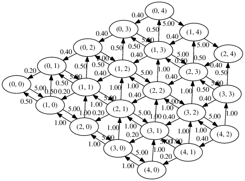
The .dot file is a standard graph
format but you can also just open up the
.ps file in whatever you want and
modify the image. Here it is in inkscape:
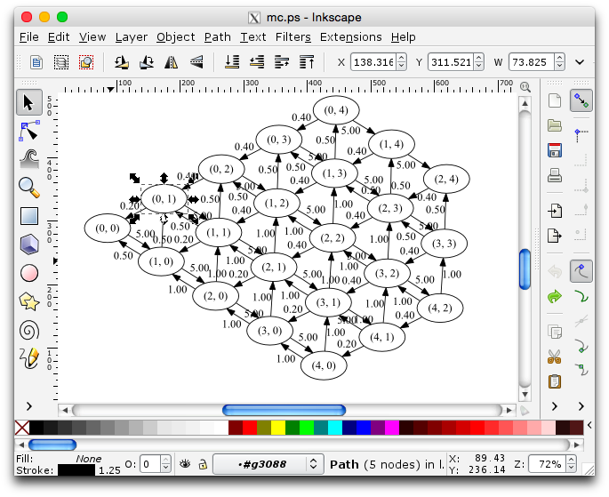
Even if the above is not as immediately esthetically pleasing as a nice Tikz diagram (but how could it be?) it’s a nice quick and easy way to visualise a Markov chain as you’re working on it.