Simulating a dice based simulation of a Markov process
I do my best to follow evidence based teaching methodologies (see for example: Freeman et al. 2014: www.pnas.org/content/111/23/8410). One topic I will be teaching this week in my game theory class is the Moran process. As an introduction to this my students will be using a variety of different sided dice (die?) to simulate the process themselves so as to understand the mathematical model. By it’s nature this process can take a while to complete, so theoretically my students could get bored by rolling a dice 40 times and not seeing anything happen. To understand what parameters would help avoid this, in this blog post I will simulate the activity (and not the Moran process itself).
The Moran process
The Moran process is a discrete mathematical model of evolution. Given a finite population \(N\) of individuals of \(n\) types, and a game \(A\in\mathbb{R}^{n\times n}\).
I will be skipping some of the details of this in this post but if you’re interesting:
- The wiki page on the Moran process: en.wikipedia.org/wiki/Moran_process
- My class notes on the topic: vknight.org/gt/chapters/12/
- My personal notes for the activity itself (these are rather brief and meant for me): vkgt.readthedocs.io/en/latest/meetings/11-moran-processes.html
The basic process follows the following steps:
- all individuals play all other individuals and obtain a fitness based on \(A\).
- an individual is selection to reproduce based on their fitness.
- an individual is randomly selected to be removed (not based on their fitness).
Here is a diagram that describes this:

This stochastic process will terminate once all individuals are of the same type.
The Moran process is both something I teach and an area of my research interests. Marc Harper, Owen Campbell, Nikoleta Glynatsi and I have a paper under review at the moment that studies this process in the setting of the Prisoner’s Dilemma (using the large number of strategies in the Axelrod-Python library). You can read the pre print here: arxiv.org/abs/1707.06920.
The activity
The activity I use in class is to have the students work on this pdf where they complete the various fitness and probability calculations in the case of:
This is a well studied game called Hawk-Dove. The basic idea here is that a single Hawk gets more resources when there are less other Hawks with which it needs to compete.
I’ve run a similar activity during school outreach visits twice. During both times, my PhD students Henry Wilde and Nikoleta Glynatsi had good reflective discussions that have resulted in how this activity looks now.
The students will in pairs work out the various probabilities:
- A hawk being selected for reproduction when there are 2 hawks: \(3/4\) and 1 Hawk: \(1/2\).
- A hawk being selection for removal when there are 2 hawks: \(2/3\) and 1 Hawk: \(1/3\).
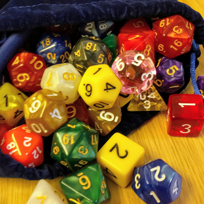
Once this is done students will use a 6 sided dice (for the \(1/2\) and \(1/3\), \(2/3\) samples) and a 4 sided dice (for the \(3/4\)) to simulate the process (any other combination of appropriately sided dice would work).
After they have done this a few times (once we arrive at 0 or 3 Hawks starting again), we’ll have a group discussion, estimating the probability of a single Hawk taking over the population and also discuss the theoretic results that let us find this probability.
To check the timing of this (perhaps the specific parameters I’ve chosen will result in the process lasting way too long?) and to double check that the dice I’m using are the right ones I have written a simulation of the activity where I get the computer to roll 6 and 4 sided dice.
The simulation
Here are the libraries we’re going to use:
import collections

import matplotlib.pyplot as plt
import numpy as np
Here is the actual simulation code:
def roll_n_sided_dice(n=6):
    """
    Roll a dice with n sides.
    """
    return np.random.randint(1, n + 1)

class MoranProcess:
    """
    A class for a moran process with a population of
    size N=3 using the standard Hawk-Dove Game:

    A =
       [0, 3]
       [1, 2]

    Note that this is a simulation corresponding to an
    in class activity where students roll dice.
    """
    def __init__(self, number_of_hawks=1, seed=None):

        if seed is not None:
            np.random.seed(seed)

        self.number_of_hawks = number_of_hawks
        self.number_of_doves = 3 - number_of_hawks

        self.dice_and_values_for_hawk_birth = {1: (6, {1, 2, 3}), 2: (4, {1, 2, 3})}
        self.dice_and_values_for_hawk_death = {1: (6, {1, 2}), 2: (6, {1, 2, 3, 4})}

        self.history = [(self.number_of_hawks, self.number_of_doves)]

    def step(self):
        """
        Select a hawk or a dove for birth.
        Select a hawk or a dove for death.

        Update history and states.
        """
        birth_dice, birth_values = self.dice_and_values_for_hawk_birth[self.number_of_hawks]
        death_dice, death_values = self.dice_and_values_for_hawk_death[self.number_of_hawks]

        select_hawk_for_birth = self.roll_dice_for_selection(dice=birth_dice, values=birth_values)
        select_hawk_for_death = self.roll_dice_for_selection(dice=death_dice, values=death_values)

        if select_hawk_for_birth:
            self.number_of_hawks += 1
        else:
            self.number_of_doves += 1

        if select_hawk_for_death:
            self.number_of_hawks -= 1
        else:
            self.number_of_doves -= 1

        self.history.append((self.number_of_hawks, self.number_of_doves))


    def roll_dice_for_selection(self, dice, values):
        """
        Given a dice and values return if the random roll is in the values.
        """
        return roll_n_sided_dice(n=dice) in values

    def simulate(self):
        """
        Run the entire simulation: repeatedly step through
        until the number of hawks is either 0 or 3.
        """
        while self.number_of_hawks in [1, 2]:
            self.step()
        return self.number_of_hawks

    def __len__(self):
        return len(self.history)
There is essentially a single Python class that does all the work (keeping track
of the number of hawks and doves at each stage), you’ll note that we
specifically self.roll_dice_for_selection which is exactly simulating what
the students will be doing.
To run this over \(10 ^ 7\) repetitions (in class I suspect we will do about 50):
>>> repetitions = 10 ** 7
>>> end_states = []
>>> path_lengths = []
>>> for seed in range(repetitions):
...     mp = MoranProcess(seed=seed)
...     end_states.append(mp.simulate())
...     path_lengths.append(len(mp))
The probability with which a Hawk takes over (“fixation probability”):
>>> counts = collections.Counter(end_states)
>>> counts[3] / repetitions
0.5452601
That’s the value we will be aiming to calculate. Here’s a quick look at how many steps (how many times they will be rolling dice) each student is likely to go through:
>>> plt.hist(path_lengths, bins=20)
>>> plt.title("Path lengths: Mean={:0.2f}, 95%={:0.2f},  80%={:0.2f}".format(np.mean(path_lengths),
...                                                                          np.percentile(path_lengths, 95),
...                                                                          np.percentile(path_lengths, 80)));
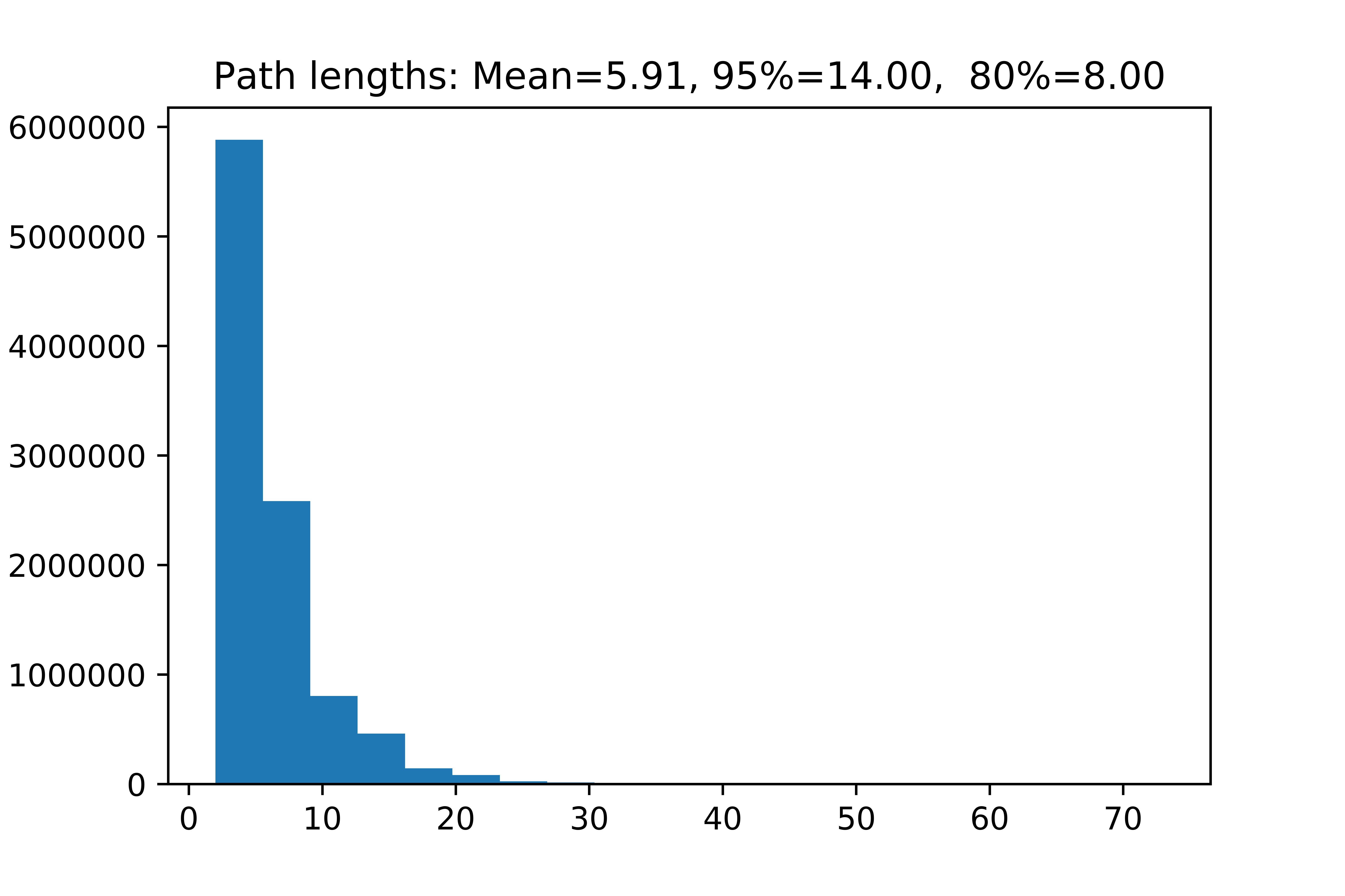
We see that on average the students will be rolling dice less than 6 times per simulation and 95% of time less than 14 times (which seems reasonable).
Note that the above is not how you would actually study this process. For example the code, whilst well written is specific for the \(N=3\) case: I actually want to hard code the dice we’ll be using. I could perhaps write something that automatically figures out what dice to use (not just in terms of how many sides but also in terms of whether or not the dice exists).
Other approaches
One way to study this analytically would be to translate the earlier calculated probabilities in to a transition matrix of a given Markov chain. In this case our transition matrix is:
In this setting \(P_{ij}\) corresponds to the probability of going from \(i\) hawks to \(j\) hawks. We note that \(P_{00}\) and \(P_{33}\) are both \(1\) which indicates that these are absorbing states.
We can then raise \(P\) to a large power to see what happens after a large number of transitions and read \((P ^ {10 ^ 2})_{13}\):
>>> P = np.array([[1, 0, 0, 0],
...              [1 / 6, 1 / 2, 1 / 3, 0],
...              [0, 1 / 6, 7 / 12, 1 / 4],
...              [0, 0, 0, 1]])
>>> np.round(np.linalg.matrix_power(P, 100)[1], 4)
array([ 0.4545,  0.    ,  0.    ,  0.5455])
We see that our large numeric simulation is not far off as the theoretic value is (after 100 steps) \(0.5455\).
The problem with this linear algebraic approach is that it is still a bit naive: it only holds for the case \(N=3\). There is thankfully a known formula for the probability which we use here:
def theoretic_fixation(N, game, i=1):
    """
    Calculate x_i
    """
    f_ones = np.array([(game[0, 0] * (i - 1) + game[0, 1] * (N - i)) / (N - 1) for i in range(1, N)])
    f_twos = np.array([(game[1, 0] * i + game[1, 1] * (N - i - 1)) / (N - 1) for i in range(1, N)])
    gammas = f_twos / f_ones
    return (1 + np.sum(np.cumprod(gammas[:i-1]))) / (1 + np.sum(np.cumprod(gammas)))
>>> theoretic_fixation(N=3, game=np.array([[0, 3], [1, 2]]), i=1)
0.54545454545454553
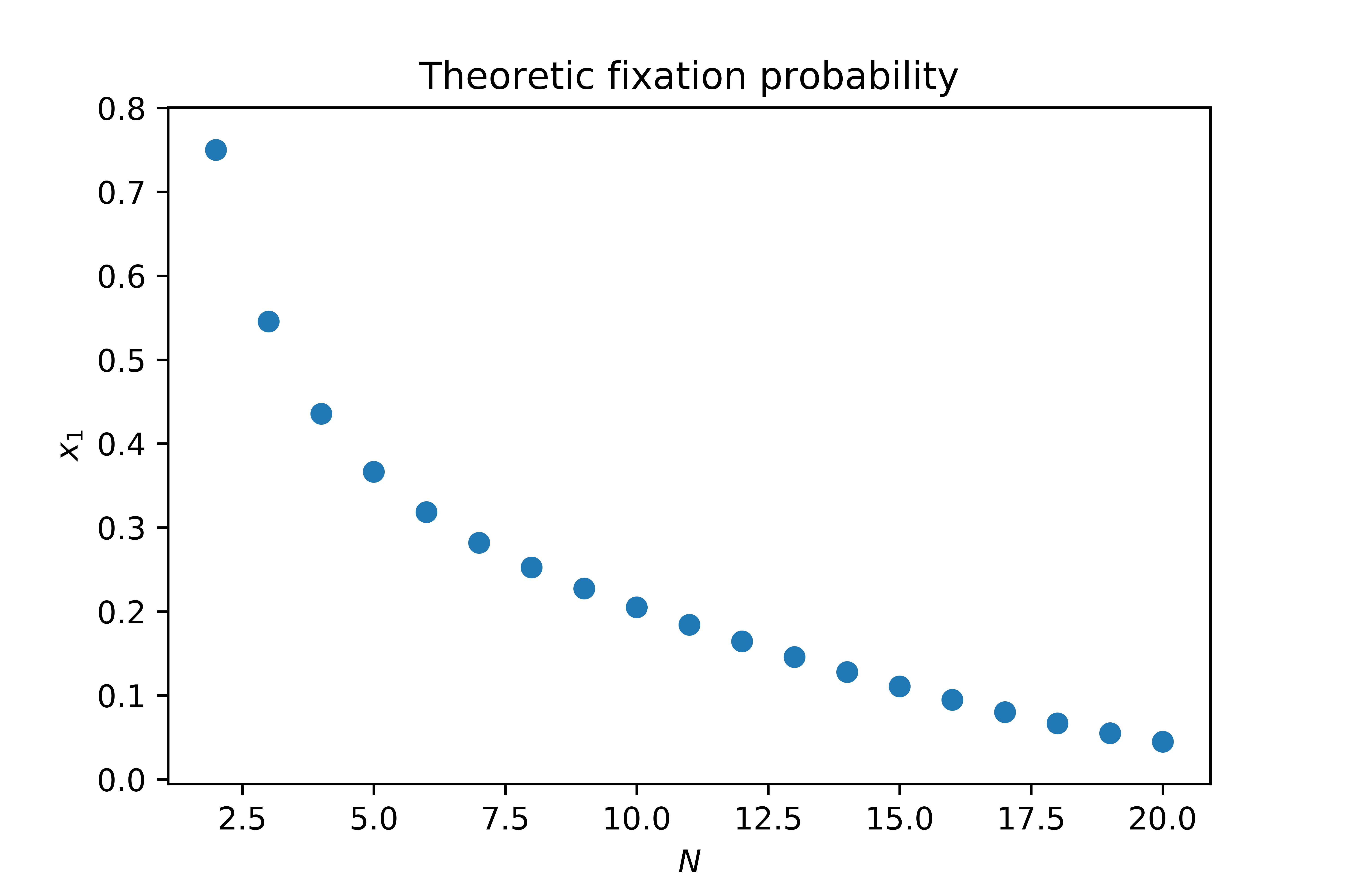
We can thus use this to see the probability of a hawk taking over a population of \(N\) doves:
>>> Ns = range(2, 20 + 1)
>>> fixations = [theoretic_fixation(N=n, game=np.array([[0, 3], [1, 2]]), i=1)
...              for n in Ns]
...              plt.scatter(Ns, fixations)
...              plt.xlabel("$N$")
...              plt.ylabel("$x_1$")
...              plt.title("Theoretic fixation probability");
This later part will form part of the in class discussion: relating the theoretic results to what the students did and highlighting how they can be used to efficiently understand a system.
I’m looking forward to trying this out in class and if nothing else, playing with different sided dice is always fun.