Playing against a mixed strategy in class
This post mirrors this post from last year in which I described how my students and I played against various mixed strategies in a modified version of matching pennies.
This is the game we played:
I wrote a sage interact that allows for a quick visualisation of a random sample from a mixed strategy.
I handed out sheets of papers on which students would input their preferred strategies (‘H’ or ‘T’) whilst I sampled randomly from 3 different mixed strategies:
- \(\sigma_1 = (.2, .8)\)
- \(\sigma_1 = (.9, .1)\)
- \(\sigma_1 = (1/3, 2/3\)
Based on the class notation that implies that the computer was the row player and the students the column player. The sampled strategies were (we played 6 rounds for each mixed strategy):
- TTHTTT
- HHHTHT
- TTTTTH
Round 1
This mixed strategy (recall \(\sigma_1=(.2,.8)\)) implies that the computer will be mainly playing T (the second strategy equivalent to the second row), and so based on the bi-matrix it is in the students interest to play H. Here is a plot of the mixed strategy played by all the students:
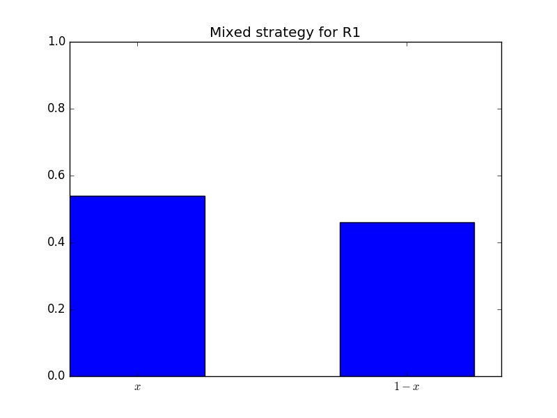
The mixed strategy played was \(\sigma_2=(.54,.46)\). Note that in fact in this particular instance that actual best response is to play \(\sigma_2=(1,0)\). This will indeed maximise the expected value of:
Indeed: the above is an increasing linear function in \(x\) so the highest value is obtained when \(x=1\).
The mean score for this round by everyone was: 1.695. The theoretical mean score (when playing the best response for six consecutive games is): \(6(-.2\times 2+.8)=2.4\), so (compared to last year) this was quite low.
Here is a distribution of the scores:
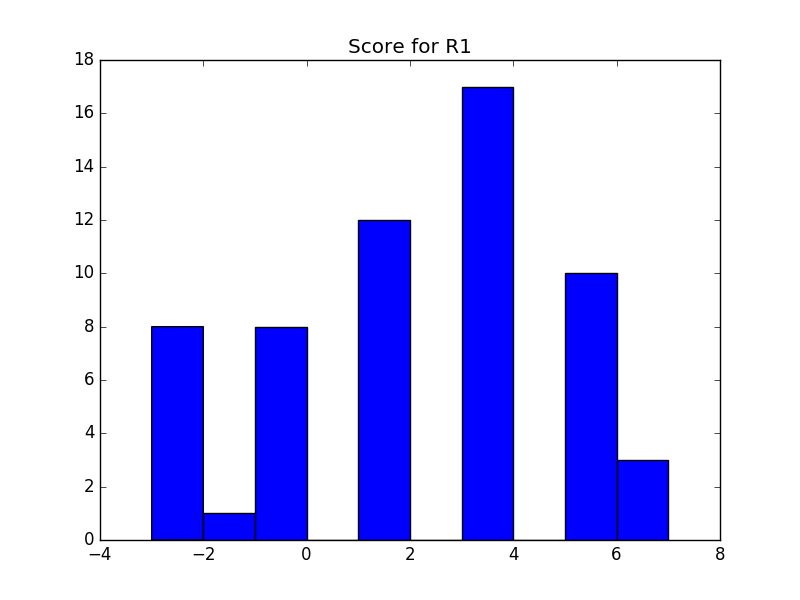
We see that a fair number of students lost but 1 student did get the highest possible score (7).
Round 2
Here the mixed strategy is \(\sigma_1=(.9,.1)\), implying that students should play T more often than H. Here is a plot of the mixed strategy played by all the students:
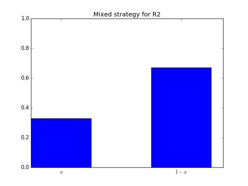
The mixed strategy played was \(\sigma_2=(0.329,0.671)\). Similarly to before this is not terribly close to the actual best response which is \((0,1)\) (due to the expected utility now being a decreasing linear function in \(x\).
Here is a distribution of the scores:
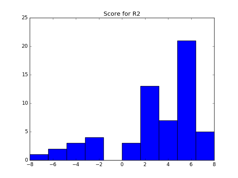
We see that some still managed to lose this round but overall mainly winners.
Round 3
Here is where things get interesting. The mixed strategy played by the computer is here \(\sigma_1=(1/3,2/3)\), it is not now obvious which strategy is worth going for!
Here is the distribution played:
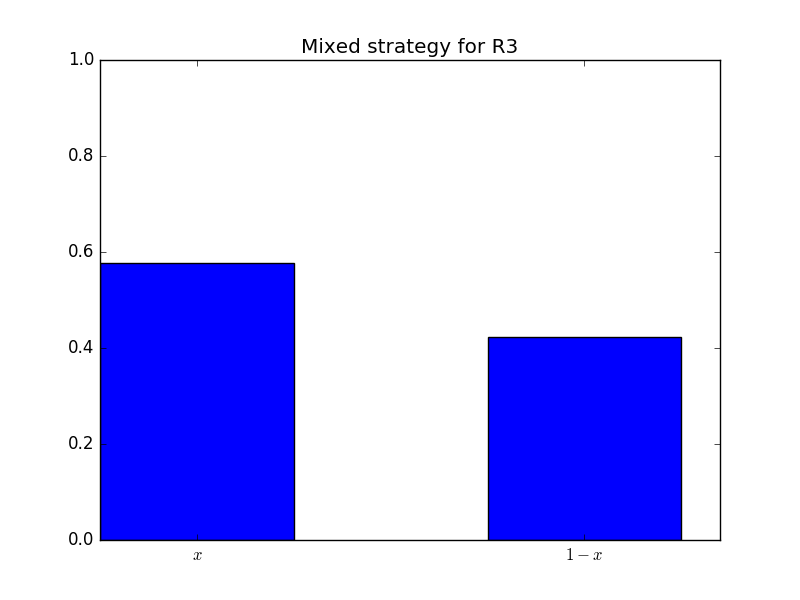
The mixed strategy is \(\sigma_2=(0.58,0.42) and the mean score was 1.11. Here is what the distribution looked like:
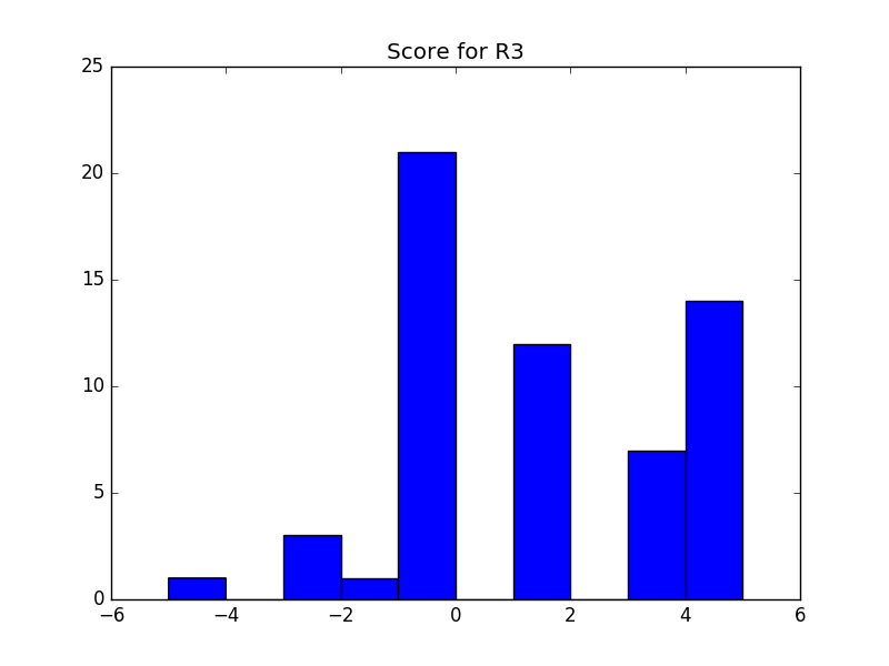
It looks like we have a few more losers than winners but not by much.