On testing degeneracy of bi-matrix games
We (James Campbell and Vince Knight are writing this together) have been working on implementing code in Sage to test if a game is degenerate or not. In this post we’ll prove a simple result that is used in the algorithm that we are/have implemented.
Bi-Matrix games
For a general overview of these sorts of things take a look at this post from a while ago on the subject of bi-matrix games in Sage. A bi-matrix is a matrix of tuples corresponding to payoffs for a 2 player Normal Form Game. Rows represent strategies for the first player and columns represent strategies for the second player, and each tuple of the bi-matrix corresponds to a tuple of payoffs. Here is an example:
We see that if the first player plays their third row strategy and the second player their second column strategy then the first player gets a utility of 6 and the second player a utility of 1.
This can also be written as two separate matrices. A matrix \(A\) for Player 1 and \(B\) for Player 2.
Here is how this can be constructed in Sage using the NormalFormGame class:
sage: A = matrix([[3,3],[2,5],[0,6]])
sage: B = matrix([[3,2],[2,6],[3,1]])
sage: g = NormalFormGame([A, B])
sage: g
Normal Form Game with the following utilities: {(0, 1): [3, 2], (0, 0): [3, 3],
(2, 1): [6, 1], (2, 0): [0, 3], (1, 0): [2, 2], (1, 1): [5, 6]}
Currently, within Sage, we can obtain the Nash equilibria of games:
sage: g.obtain_nash()
[[(0, 1/3, 2/3), (1/3, 2/3)], [(4/5, 1/5, 0), (2/3, 1/3)], [(1, 0, 0), (1, 0)]]
We see that this game has 3 Nash equilibria. For each, we see that the supports (the number of non zero entries) of both players’ strategies are the same size. This is, in fact, a theoretical certainty when games are non degenerate.
If we modify the game slightly:
sage: A = matrix([[3,3],[2,5],[0,6]])
sage: B = matrix([[3,3],[2,6],[3,1]])
sage: g = NormalFormGame([A, B])
sage: g.obtain_nash()
[[(0, 1/3, 2/3), (1/3, 2/3)], [(1, 0, 0), (2/3, 1/3)], [(1, 0, 0), (1, 0)]]
We see that the second equilibrium has supports of different sizes. In fact, if the first player did play \((1,0,0)\) (in other words just play the first row) the second player could play any mixture of strategies as a best response and not particularly \((2/3,1/3)\). This is because the game in consideration is now degenerate.
(Note that both of the games above are taken from Nisan et al. 2007 [pdf].)
What is a degenerate game
A bimatrix game is called nondegenerate if the number of pure best responses to a mixed strategy never exceeds the size of its support. In a degenerate game, this definition is violated, for example if there is a pure strategy that has two pure best responses (as in the example above), but it is also possible to have a mixed strategy with support size \(k\) that has \(k+1\) strategies that are a best response.
Here is an example of this:
If we consider the mixed strategy for player 2: \(y=(1/2,1/2)\), then the utility to player 1 is given by:
We see that there are 3 best responses to \(y\) and as \(y\) has support size 2 this implies that the game above is degenerate.
What does the literature say about degenerate games
The original definition of degenerate games was given in Lemke, Howson 1964 [pdf] and their definition was dependent on the labeling polytope that they used for their famous algorithm for the computation of equilibria (which is currently being implemented in Sage!). Further to this Stengel 1999 [ps] offers a nice overview of a variety of equivalent definitions.
Sadly, all of these definitions require finding a particular mixed strategy profile \((x, y)\) for which a particular condition holds. To be able to implement a test for degeneracy based on any of these definitions would require a continuous search over possible mixed strategy pairs.
In the previous example (where we take \(y=(1/2,1/2)\) we could have identified this \(y\) by looking at the utilities for each pure strategy for player 1 against \(y=(y_1, 1-y_1)\):
(\(r_i\) denotes row strategy \(i\) for player 1.) A plot of this is shown:

We can (in this instance) quickly search through values of \(y_1\) and identify the point that has the most best responses which gives the best chance of passing the degeneracy condition (\(y_1=1/2\)). This is not really practical from a generic point of view which leads to this blog post: we have identified what the particular \(x, y\) is that is sufficient to test.
A sufficient mixed strategy to test for degeneracy
The definition of degeneracy can be written as:
Def. A Normal Form Game is degenerate iff:
There exists \(x\in \Delta X\) such that \( |S(x)| < |\sigma_2| \) where \(\sigma_2\) is the support such that \( (xB)_j = \max(xB) \), for all \(j \) in \( \sigma_2\).
OR
There exists \(y\in \Delta Y\) such that \( |S(x)| < |\sigma_1| \) where \(\sigma_1\) is the support such that \( (Ay)_i = \max(Ay) \), for all \(i \) in \( \sigma_1\).
(\(X\) and \(Y\) are the pure strategies for player 1 and 2 and \(\Delta X, \Delta Y\) the corresponding mixed strategies spaces.
The result we are implementing in Sage aims to remove the need to search particular mixed strategies \(x, y\) (a continuous search) and replace that by a search over supports (a discrete search).
Theorem. A Normal Form Game is degenerate iff:
There exists \( \sigma_1 \subseteq X \) and \( \sigma_2 \subseteq Y \) such that \( |\sigma_1| < |\sigma_2| \) and \( S(x^*) = \sigma_1 \) where \( x^* \) is a solution of \( (xB)_j = \max(xB) \), for all \(j \) in \( \sigma_2 \) (note that a valid \(x^*\) is understood to be a mixed strategy vector).
OR
There exists \( \sigma_1 \subseteq X \) and \( \sigma_2 \subseteq Y \) such that \( |\sigma_1| > |\sigma_2| \) and \( S(y^*) = \sigma_2 \) where \( y^* \) is a solution of \( (Ay)_i = \max(Ay) \), for all \(i \) in \( \sigma_1 \).
Using the definition given above the proof is relatively straightforward but we will include it below (mainly to try and convince ourselves that we haven’t made a mistake).
We will only consider the first part of each condition (the ones for the first player). The result follows in the same way for the second player.
Proof \(\Leftarrow\)
Assume a game defined by \(A, B\) is degenerate, by the above definition without loss of generality this implies that there exists an \(x\in \Delta X\) such that \( |S(x)| < |\sigma_2| \) where \(\sigma_2\) is the support such that \( (xB)_j = \max(xB) \), for all \(j \) in \( \sigma_2\).
If we denote \(S(x)\) by \(\sigma_1\) then the definition implies that \(|\sigma_1| < |\sigma_2| \) and further more that \( (xB)_j = \max(xB) \), for all \(j \) in \( \sigma_2 \) as required.
Proof \(\Rightarrow\)
If we now assume that we have \(\sigma_1, \sigma_2, x^*\) as per the first part of the theorem then we have \(|\sigma_1|<|\sigma_2|\) and taking \(x=x^*\) implies that \(|S(x)|<|\sigma_2|\). Furthermore as \(x^*\) is a solution of \( (xB)_j = \max(xB) \) the result follows (by the definition given above).
Implementation
This result implies that we simply need to consider all potential pairs of supports. Depending on the relative size of the supports we can use one of the two conditions of the result. If we ordered the supports by size the situation for the two player game looks somewhat like this:
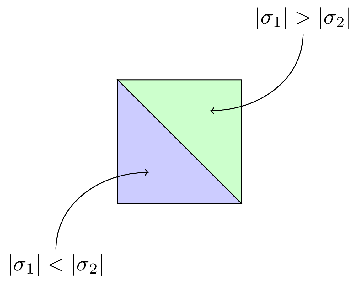
Note that for an \(m\times n\) game there are \((2^m-1)\) potential supports for player 1 (the size of the powerset of strategy set without the empty set) and \((2^n-1)\) potential supports of for player 2. Thus the rectangle drawn above has dimension \((2^m-1)\times(2^n-1)\). Needless to say that our implementation will not be efficient (testing degeneracy is after all an NP complete problem in linear programming (see Chandrasekaran 1982 - [pdf]) but at least we have identified exactly which mixed strategy we need to test for each support pair.
References
- Chandrasekaran, R., Santosh N. Kabadi, and Katta G. Murthy. “Some NP-complete problems in linear programming.” Operations Research Letters 1.3 (1982): 101-104. [pdf]
- Lemke, Carlton E., and Joseph T. Howson, Jr. “Equilibrium points of bimatrix games.” Journal of the Society for Industrial & Applied Mathematics 12.2 (1964): 413-423. [pdf]
- N Nisan, T Roughgarden, E Tardos, VV Vazirani Vol. 1. Cambridge: Cambridge University Press, 2007. [pdf]
- von Stengel, B. “Computing equilibria for two person games.” Technical report. [ps]