Python, natural language processing and predicting funny
Every year there is a big festival in Edinburgh called the fringe festival. I blogged about this a while ago, in that post I did a very basic bit of natural language processing aiming to try and identify what made things funny. In this blog post I’m going to push that a bit further by building a classification model that aims to predict if a joke is funny or not. (tldr: I don’t really succeed but but that’s mainly because I have very little data - having more data would not necessarily guarantee success either but the code and approach is what’s worth taking from this post… 😪).
If you want to skip the brief description and go straight to look at the code you can find the ipython notebook on github here and on cloud.sagemath here.
The data comes from a series of BBC articles which reports (more or less every year since 2011?) the top ten jokes at the fringe festival. This does in fact only give 60 odd jokes to work with…
Here is the latest winner (by Tim Vine):
I decided to sell my Hoover… well it was just collecting dust.
After cleaning it up slightly I’ve thrown that all in a json file here.
So in order to import the data in to a panda data frame I just run:
import pandas
df = pandas.read_json('jokes.json') # Loading the json file
Pandas is great, I’ve been used to creating my own bespoke classes for handling
data but in general just using pandas does the exact right job.
At this point I basically follow along with
this post on sentiment analysis of twitter which makes use of the ridiculously powerful nltk library.
We can use the nltk library to ‘tokenise’ and get rid of common words:
commonwords = [e.upper() for e in set(nltk.corpus.stopwords.words('english'))] # <- Need to download the corpus: import nltk; nltk.download()
commonwords.extend(['M', 'VE'])  # Adding a couple of things that need to be removed
tokenizer = nltk.tokenize.RegexpTokenizer(r'\w+')  # To be able to strip out unwanted things in strings
string_to_list = lambda x: [el.upper() for el in tokenizer.tokenize(x) if el.upper() not in commonwords]
df['Joke'] = df['Raw_joke'].apply(string_to_list)
Note that this requires downloading one of the awesome corpuses (thats apparently the right way to say that) from nltk.
Here is how this looks:
joke = 'I decided to sell my Hoover... well it was just collecting dust.'
string_to_list(joke)
which gives:
['DECIDED', 'SELL', 'HOOVER', 'WELL', 'COLLECTING', 'DUST']We can now get started on building a classifier
Here is the general idea of what will be happening:

First of all we need to build up the ‘features’ of each joke, in other words pull the words out in to a nice easy format.
To do that we need to find all the words from our training data set, another way of describing this is that we need to build up our dictionary:
df['Year'] = df['Year'].apply(int)

def get_all_words(dataframe):
    """
    A function that gets all the words from the Joke column in a given dataframe
    """
    all_words = []
    for jk in dataframe['Joke']:
        all_words.extend(jk)
    return all_words

all_words = get_all_words(df[df['Year'] <= 2013])  # This uses all jokes before 2013 as our training data set.
We then build something that will tell us for each joke which of the overall words is in it:
def extract_features(joke, all_words):
    words = set(joke)
    features = {}
    for word in words:
        features['contains(%s)' % word] = (word in all_words)
    return features
Once we have done that, we just need to decide what we will call a funny joke. For this purpose
We’ll use a funny_threshold and any joke that ranks above the
funny_threshold in any given year will be considered funny:
funny_threshold = 5
df['Rank'] = df['Rank'].apply(int)
df['Funny'] = df['Rank'] <= funny_threshold
Now we just need to create a tuple for each joke that puts the features mentioned earlier and a classification (if the joke was funny or not) together:
df['Labeled_Feature'] = zip(df['Features'],df['Funny'])We can now (in one line of code!!!!) create a classifier:
classifier = nltk.NaiveBayesClassifier.train(df[df['Year'] <= 2013]['Labeled_Feature'])This classifier will take into account all the words in a given joke and spit out if it’s funny or not. It can also give us some indication as to what makes a joke funny or not:
classifier.show_most_informative_features(10)Here is the output of that:
Most Informative Features
     contains(GOT) = True   False : True   =  2.4 : 1.0
    contains(KNOW) = True    True : False  =  1.7 : 1.0
  contains(PEOPLE) = True   False : True   =  1.7 : 1.0
     contains(SEX) = True   False : True   =  1.7 : 1.0
   contains(NEVER) = True   False : True   =  1.7 : 1.0
      contains(RE) = True    True : False  =  1.6 : 1.0
  contains(FRIEND) = True    True : False  =  1.6 : 1.0
     contains(SAY) = True    True : False  =  1.6 : 1.0
  contains(BOUGHT) = True    True : False  =  1.6 : 1.0
     contains(ONE) = True    True : False  =  1.5 : 1.0
This immediately gives us some information:
- If your joke is about
SEXis it more likely to not be funny. - If your joke is about
FRIENDs is it more likely to be funny.
That’s all very nice but we can now (theoretically - again, I really don’t have enough data for this) start using the mathematical model to tell you if something is funny:
joke = 'Why was 10 afraid of 7? Because 7 8 9'
classifier.classify(extract_features(string_to_list(joke), get_all_words(df[df['Year'] <= 2013])))
That joke is apparently funny (the output of above is True). The following joke however is apparently not (the output of below if False):
joke = 'Your mother is ...'
print classifier.classify(extract_features(string_to_list(joke), get_all_words(df[df['Year'] <= 2013])))
As you can see in the ipython notebook it is then very easy to measure how good the predictions are (I used the data from years before 2013 to predict 2014).
Results
Here is a plot of the accuracy of the classifier for changing values of funny_threshold:
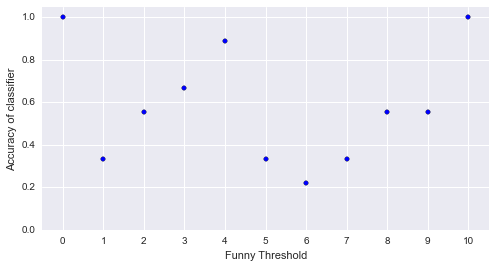
You’ll notice a couple of things:
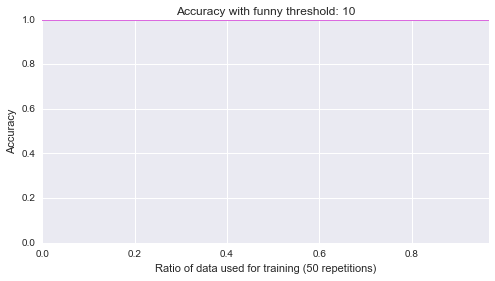
- When the threshold is 0 or 1: the classifier works perfectly. This makes sense: all the jokes are either funny or not so it’s very easy for the classifier to do well.
- There seems to be a couple of regions where the classifier does particularly poorly: just after a value of 4. Indeed there are points where the classifier does worse than flipping a coin.
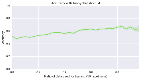
- At a value of 4, the classifier does particularly well!
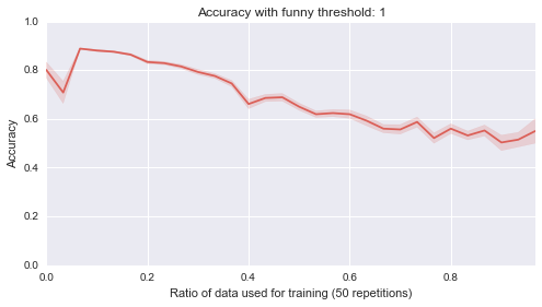
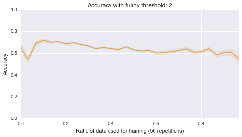
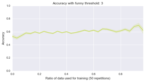
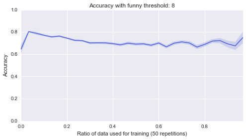
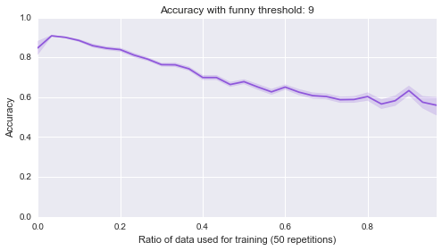
Now, one final thing I’ll take a look at is what happens if I start randomly selecting a portion of the entire data set to be the training set:

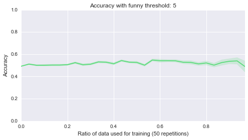
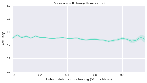
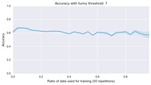
Below are 10 plots that correspond to 50 repetitions of the above where I randomly sample a ratio of the data set to be the training set:
Finally (although it’s really not helpful), here are all of those on a single plot:
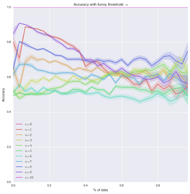
First of all: all those plots are basically one line of seaborn code which is ridiculously cool. Seaborn is basically magic:
sns.tsplot(data, steps)Second of all, it looks like the lower bound of the classifiers is around .5. Most of them start of at .5, in other words they are as good as flipping a coin before we let them learn from anything, which makes sense. Finally it seems that the threshold of 4 classifier seems to be the only one that gradually improves as more data is given to it. That’s perhaps indicating that something interesting is happening there but that investigation would be for another day.
All of the conclusions about the actual data should certainly not be taken seriously: I simply do not have enough data. But, the overall process and code is what is worth taking away. It’s pretty neat that the variety of awesome python libraries lets you do this sort of thing more or less out of the box.
Please do take a look at this github repository
but I’ve also just put the notebook on cloud.sagemath so assuming you
pip install the libraries and get the data etc you can play around with this right in your browser: