Replicator dynamics

In class we talked through a way of modelling emergent behaviour: we all took on the roles or Rocks, Paper or Scissors.

You can see a recording of this here.

We used the following representation of Rock Paper Scissors.

\[M_r = \begin{pmatrix} 0 & -1 & 1 \\ 1 & 0 & -1 \\ -1 & 1 & 0 \\ \end{pmatrix}\]

This is was our first time being interested in modelling a population. We roughly counted the proportion of Rocks, Papers and Scissors (you all got to choose) in the class and came up with the population vector:

\[x = (.42, .38, .20)\]

From this, we computed the expected fitness of each type of individual assuming they’d need to interact with everyone else in the population:

You can see the various calculations here:

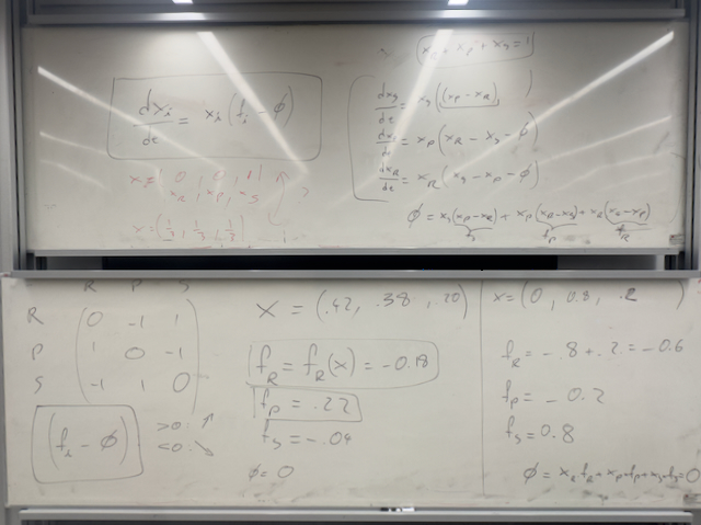
Following this we discussed how the types with low fitness would change their type. In this case: the Rocks want to change to be Paper.

We calculated the average fitness:

\[\phi = x_R f_R + x_P f_P + x_S f_S\]

and that gave as a way to more clearly describe “low”: as below average.

Note that in rock paper scissors the average will always be zero but this is not always the case.

This lead to us describing the situation where the proportion of a given type goes up:

\[f_i > \phi\]

Or the proportion of a given type goes down:

\[f_i < \phi\]

This leads to the Replicator Dynamics Equation which in our case is in fact 3 differential equations. One for each of the types.

We talked briefly about stability and I discussed what is called Evolutionary Stability which is a population that remains stable even when a mutant enters.

I showed how to use Nashpy to solve the differential equations numerically and you can find the notebook I used to do that here.