Overview of Numerical Integration
In today’s class we spoke about numerical integration: a term used to refer to techniques that deal with numerical solution to differential equations.
You can the recording here.
We started the class by having a discussion of what we had seen so far in the course:
We have seen:
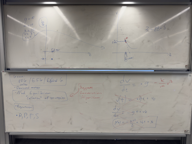
- Different types of Games:
- Normal Form Games
- Extensive Form Games
- Repeated Games
- Dominated Strategies which is when a strategy is never rationally played. We did not specifically list it but also in this category is the notion of a best response.
- Nash Equilibium and the Support Enumeration Algorithm.
- Reputation and the Iterated Prisoner’s Dilemma
Now whilst that summary is not exhaustive of everything covered in the chapters seen so far it is a good list to scaffold your independent study.
After that we spoke about Numerical integration.
Specifically I asked you to write out the solution to the following differential equation:
\[\frac{dv}{dt} = - g\]Actually, I asked you first what that was: an equation for something falling under the effect of gravity.
We were quickly able to arrive at:
\[v(t) = -g t + v_0\]And in turn get the vertical displacement as:
\[y(t) = -g t ^ 2 / 2 + v_0 t + y_0\]I then asked what was wrong with this and Peter correctly brought up air resistance. Indeed, with air resistance (which is in fact very rarely negligible in practice) the differential equation is:
\[\frac{dv}{dt} = - g - \frac{k}{m}v^2\]This is not an equation we can find a closed form solution for which leads us to the topic of this chapter: Numerical Integration.
In practice when solving differential equations numerically we can use a variety of numerical techniques to “step through time” and use the derivative as the value of the slope over a small time increment.
We talked about this and arrived essentially at Euler’s algorithm which allows us to do this.
This will be a useful tool for the next Chapter of the course which is to study evolution using a differential equation.