Un peu de math

Use the stationary distribution of an absorbing markov chain to simulate a Galton board

Simulating a Galton board with Markov chains, eigenvalues and Python

2018-11-26

The galton board (also sometimes called a "Bean machine") is a lovely way of visualising the normal distribution.

This can be modelled mathematically using Markov chains.

We first need to set up the state space we're going to use. Here is a small diagram showing how it will be done:

Responsive image

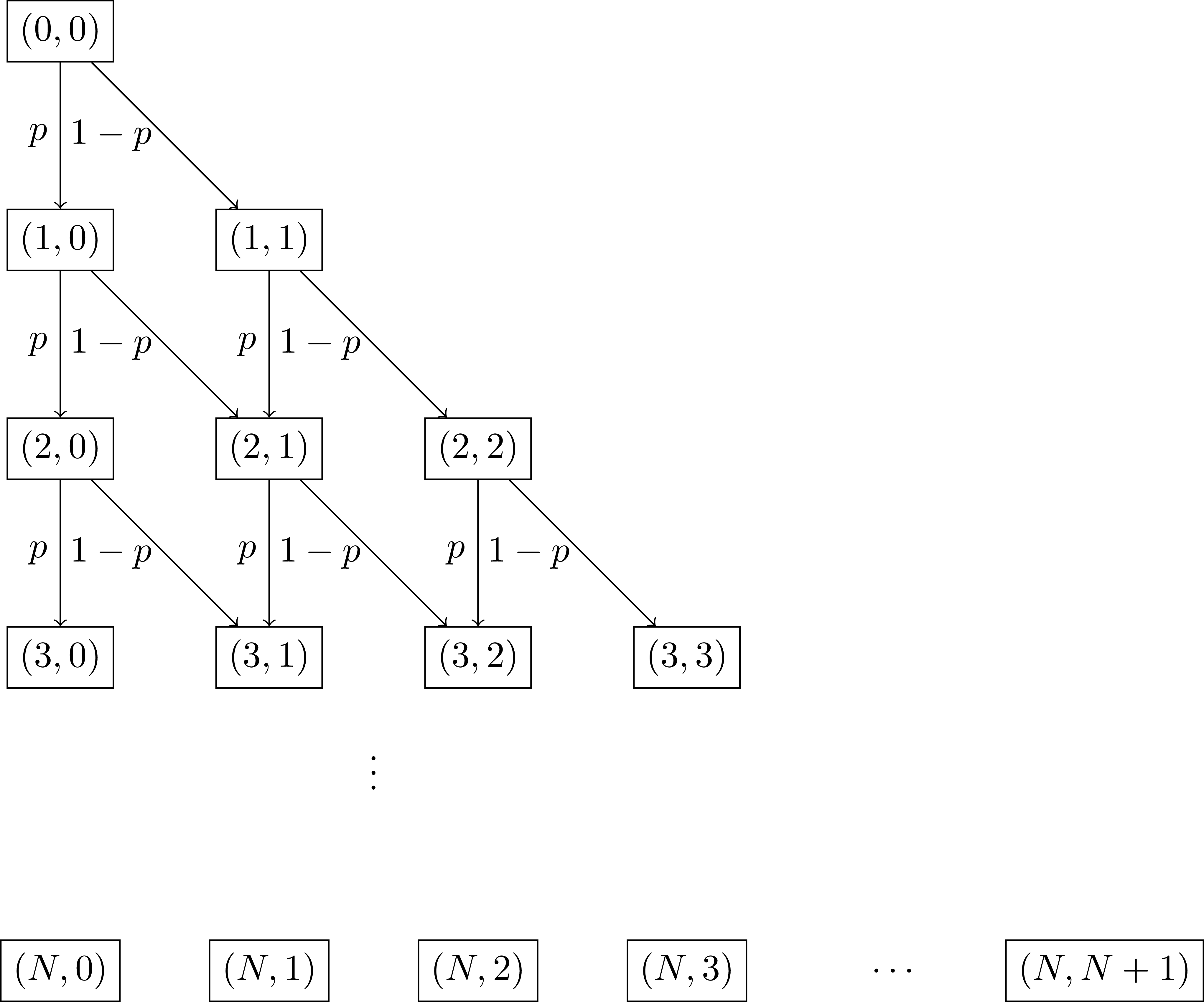
There are a few things there that don't look immediately like the usual galton board:

It is essentially rotated: this is purely to make the mathematical formulation simpler.
There is a probability $p$: this is to play with later, it is taken as the probability of a given bead to fall to the left when hitting an obstacle. In the usual case: $p=1/2$.
We limit our number of rows of obstacles to $N$.

Using this, our state space can be written as:

$$ S = \{(i, j) \in \mathbb{R}^2| 0 \leq i \leq N, 0 \leq j \leq i\} $$

A straight forward combinatorial argument gives:

$$ |S| = \binom{N + 1}{2} = \frac{(N + 1)(N + 2)}{2} $$

We are going to use Python throughout this blog post to explore the mathematical objects as we go. First let us create a python generator to create our states and also a function to get the size of the state space efficiently:

In [2]:

import numpy as np

def all_states(number_of_rows):
    for i in range(number_of_rows + 1):
        for j in range(i + 1):
            yield np.array([i, j])
            
def get_number_of_states(number_of_rows):
    return int((number_of_rows + 1) * (number_of_rows + 2) / 2)

In [3]:

list(all_states(number_of_rows=4))

Out[3]:

[array([0, 0]),
 array([1, 0]),
 array([1, 1]),
 array([2, 0]),
 array([2, 1]),
 array([2, 2]),
 array([3, 0]),
 array([3, 1]),
 array([3, 2]),
 array([3, 3]),
 array([4, 0]),
 array([4, 1]),
 array([4, 2]),
 array([4, 3]),
 array([4, 4])]

We can test that we have the correct count:

In [4]:

for number_of_rows in range(10):
    assert len(list(all_states(number_of_rows=number_of_rows))) == get_number_of_states(number_of_rows=number_of_rows)

Now that we have our state space, to fully define our Markov chain we need to define our transitions. Given two elements $s^{(1)}, s^{(2)}\in S$ we have:

$$ P_{s^{(1)}, s^{(2)}} = \begin{cases} p & \text{ if }s^{(2)} - s^{(1)} = (1, 0)\text{ and }{s_1^{(2)}} < N \\ 1 - p & \text{ if }s^{(2)} - s^{(1)} = (1, 1)\text{ and }{s_1^{(2)}} < N \\ 1 & \text{ if }s^{(2)} = N\\ 0 & \text{otherwise} \\ \end{cases} $$

The first two values ensure the beads bounce to the left and right accordingly and the third line ensures the final row is absorbing (the beads stay put once they've hit the bottom).

Here's some Python code that replicates this:

In [5]:

def transition_probability(in_state, out_state, number_of_rows, probability_of_falling_left):
    
    if in_state[0] == number_of_rows and np.array_equal(in_state, out_state):
        return 1
    
    if np.array_equal(out_state - in_state, np.array([1, 0])):
        return probability_of_falling_left
    
    if np.array_equal(out_state - in_state, np.array([1, 1])):
        return 1 - probability_of_falling_left
    
    return 0

We can use the above and the code to get all states to create the transition matrix:

In [6]:

def get_transition_matrix(number_of_rows, probability_of_falling_left):
    
    number_of_states = get_number_of_states(number_of_rows=number_of_rows)
    P = np.zeros((number_of_states, number_of_states))
    
    for row, in_state in enumerate(all_states(number_of_rows=number_of_rows)):
        for col, out_state in enumerate(all_states(number_of_rows=number_of_rows)):   
            P[row, col] = transition_probability(in_state, out_state, number_of_rows, probability_of_falling_left)
    
    return P

In [7]:

P = get_transition_matrix(number_of_rows=3, probability_of_falling_left=1/2)
P

Out[7]:

array([[ 0. ,  0.5,  0.5,  0. ,  0. ,  0. ,  0. ,  0. ,  0. ,  0. ],
       [ 0. ,  0. ,  0. ,  0.5,  0.5,  0. ,  0. ,  0. ,  0. ,  0. ],
       [ 0. ,  0. ,  0. ,  0. ,  0.5,  0.5,  0. ,  0. ,  0. ,  0. ],
       [ 0. ,  0. ,  0. ,  0. ,  0. ,  0. ,  0.5,  0.5,  0. ,  0. ],
       [ 0. ,  0. ,  0. ,  0. ,  0. ,  0. ,  0. ,  0.5,  0.5,  0. ],
       [ 0. ,  0. ,  0. ,  0. ,  0. ,  0. ,  0. ,  0. ,  0.5,  0.5],
       [ 0. ,  0. ,  0. ,  0. ,  0. ,  0. ,  1. ,  0. ,  0. ,  0. ],
       [ 0. ,  0. ,  0. ,  0. ,  0. ,  0. ,  0. ,  1. ,  0. ,  0. ],
       [ 0. ,  0. ,  0. ,  0. ,  0. ,  0. ,  0. ,  0. ,  1. ,  0. ],
       [ 0. ,  0. ,  0. ,  0. ,  0. ,  0. ,  0. ,  0. ,  0. ,  1. ]])

Once we have done this we are more of less there. With $\pi=(1,...0)$, the product: $\pi P$ gives the distribution of our beads after they drop past the first row. Thus the following gives us the final distribution over all the states after the beads get to the last row:

$$ \pi P ^ N $$

Here is some Python code that does exactly this:

In [8]:

def expected_bean_drop(number_of_rows, probability_of_falling_left):
    
    number_of_states = get_number_of_states(number_of_rows)
    pi = np.zeros(number_of_states)
    pi[0] = 1
    P = get_transition_matrix(number_of_rows=number_of_rows, probability_of_falling_left=probability_of_falling_left)
    
    return (pi @ np.linalg.matrix_power(P, number_of_rows))[-(number_of_rows + 1):]

In [9]:

expected_bean_drop(number_of_rows=3, probability_of_falling_left=1/2)

Out[9]:

array([ 0.125,  0.375,  0.375,  0.125])

We can then plot this (using matplotlib):

In [10]:

import matplotlib.pyplot as plt

def plot_bean_drop(number_of_rows, probability_of_falling_left, label=None, color=None):
    plt.plot(expected_bean_drop(number_of_rows=number_of_rows,
                                probability_of_falling_left=probability_of_falling_left),
             label=label, color=color)
    return plt

Let us use this to plot over $N=30$ rows and also overlay with the normal pdf:

In [11]:

from scipy.stats import norm

plt.figure()
plot_bean_drop(number_of_rows=30, probability_of_falling_left=1 / 2)
plt.ylabel("Probability")
plt.xlabel("Bin position");

We can also plot this for a changing value of $p$:

In [12]:

from matplotlib import cm

number_of_rows = 30

plt.figure()

for p in np.linspace(0, 1, 10):
    plot_bean_drop(
        number_of_rows=number_of_rows, 
        probability_of_falling_left=p, 
        label=f"p={p:0.02f}", 
        color=cm.viridis(p)
    )
    
plt.ylabel("Probability")
plt.xlabel("Bin position")
plt.legend();

We see that as the probability of falling left moves from 0 to 1 the distribution slow shifts across the bins.

A blog about programming (usually scientific python), mathematics (usually game theory) and learning (usually student centred pedagogic approaches).

Source code: drvinceknight Twitter: @drvinceknight Email: [email protected] Powered by: Python mathjax highlight.js Github pages Bootstrap