SAS Chapter 5 - Further packages
In this chapter we will examine three particular procedures in SAS.
- proc sql: a procedure allowing for the use of sql syntax in SAS;
- proc fcmp: a procedure allowing for the creation of custom functions;
- proc optmodel: a package that allows for optimisation in SAS.
5.1 Proc sql
5.1.1 Basic SQL
SQL is a language designed for querying and modifying databases. Used by a variety of database management software suites:
- Oracle
- Microsoft ACCESS
- SPSS
SQL uses one or more objects called TABLES where: rows contain records (observations) and columns contain variables. Importantly,
- Starts with proc sql; (as expected)
- Ends with quit; (some interactive procedures do)
The following code creates a data set called test in the work library as a copy of the mat013.mmm data set:
proc sql;
create table test as
select *
from mat013.mmm;
quit;
The "*" command tells SAS to take all variables from mat013.mmm. We can however specify exactly what variables we want:
proc sql;
create table test as
select Name, Age, Sex
from mat013.mmm;
quit;
We can also create new variables:
proc sql;
create table test as
select Name, Age, Sex, weight_in_kg/(height_in_metres**2) as bmi
from mat013.mmm;
quit;
5.1.2 Further SQL
In this section we'll take a look at what else SAS can do. For the purpose of the following examples let's write a new data set:
data mat013.example;
input Var1 $ Var2 Var3 $ Var 4 Var5 $;
cards;
A 1 A 2 B
A 1 A 2 B
B 1 A 1 C
C 2 B 2 D
C 2 C 1 E
;
run;
Some simple SQL code very easily helps us to get rid of duplicate rows (this can be very helpful when handling real data). To do this we use the "distinct" keyword.
proc sql;
create table example as
select distinct *
from mat013.example;
quit;
We can also select particular variables:
proc sql;
create table example as
select distinct var1, var2, var3
from mat013.example;
quit;
We can also use the "where" statement to select variables that obey a particular condition:
proc sql;
create table example as
select *
from mat013.example
where var2<=var4;
quit;
We can sort data sets using the "order by" keyword:
proc sql;
create table example as
select distinct *
from mat013.example
order by var1;
quit;
A very nice application of SQL is in the aggregation of summary statistics. The following code creates a new variable that gives the average value of var2. The value of this variable is the same for all the observations:
proc sql;
create table example as
select * mean(var2) as average_of_var2
from mat013.example;
quit;
We could however get something a bit more useful by aggregating the data using a "group" statement:
proc sql;
create table example as
select var1, mean(var2) as average_of_var2
from mat013.example
group by var1;
quit;
5.1.3 Joining tables with SQL
A very common use of SQL within SAS is to carry out "joins" which are equivalent to a merger of data sets. There are 4 types of joins to consider:
- inner join
- output table only contains rows common to all tables
- variable attributes taken from left most table
- outer join left
- output table contains all rows contributed by the left table
- variable attributes taken from left most table
- outer join right
- output table contains all rows contributed by the right table
- variable attributes taken from right most table
- outer join full
- output table contains all rows contributed by all tables
- variable attributes taken from left most table
To work with these examples let's use the data sets created with the following code:
data mat013.dogs;
input Owner $ Name $;
cards;
Jeff Ruffus
Janet Sam
Paul .
Joanna .
;
run;

data mat013.cats;
input Owner $ Name $;
cards;
Jeff Kitty
Paul .
Joanna Tinkerbell
Vince Chick
;
run;
The following code carries out an inner join of these two datasets also changing the name of the "Name" variable depending on which data set it was from, the output of which is shown.
proc sql;
create table merged_table as
select a.Owner,a.Name as Dog_Name, b.Name as cat_Name
from mat013.dogs as a, mat013.cats as b
where a.Owner=b.Owner;
quit;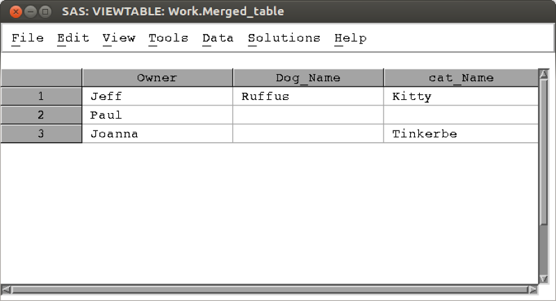
The following code carries out a left outer join, the output of which is shown.
proc sql;
create table merged_table as
select a.Owner,a.Name as Dog_Name, b.Name as cat_Name
from mat013.dogs as a
left join mat013.cats as b
on a.Owner=b.Owner;
quit;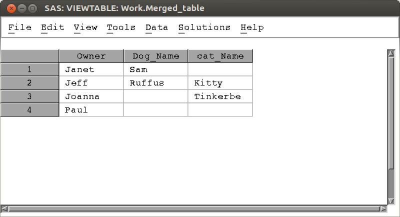
The following code carries out a right outer join, the output of which is shown.
proc sql;
create table merged_table as
select a.Owner,a.Name as Dog_Name, b.Name as cat_Name
from mat013.dogs as a
right join mat013.cats as b
on a.Owner=b.Owner;
quit;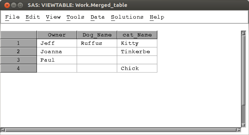
The following code carries out a full outer join, the output of which is shown.
proc sql;
create table merged_table as
select a.Owner,a.Name as Dog_Name, b.Name as cat_Name
from mat013.dogs as a
full join mat013.cats as b
on a.Owner=b.Owner;
quit;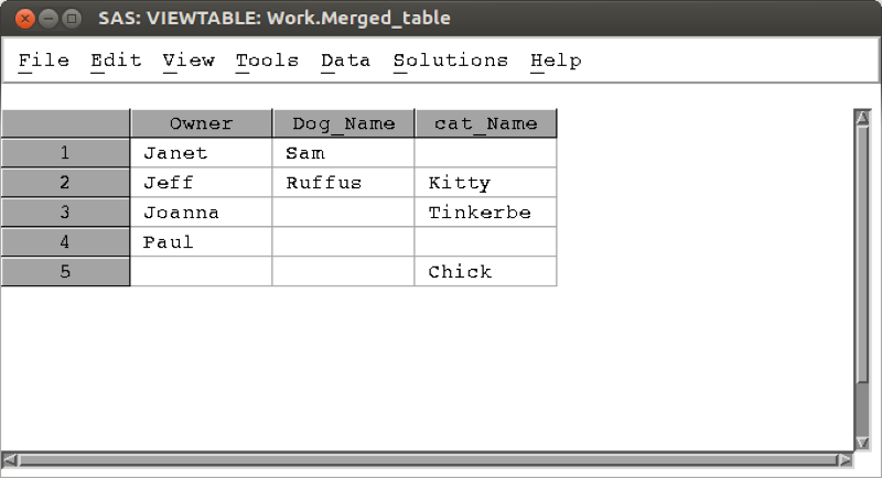
5.2 Proc fcmp
In previous chapters we have seen various in built functions in SAS. For various reasons it might be required to create a custom function. We will do this with the "fcmp" procedure. This procedure allows us to create custom functions using data step syntax (which allows for "if" and "do" statements to be used). The following code creates a function called "ln" that gives the natural log of a number:
proc fcmp outlib=sasuser.funcs.ln;
function ln(x);
y=log(x);
return(y);
endsub;
quit;
This code in fact creates a function named "ln" in a package named "funcs". The package is stored in the data set sasuser.funcs. To use this function we need to tell SAS which data set contains the function. We do this with the following piece of code:
option cmplib=sasuser.funcs;It is then straightforward to call this function:
option cmplib=sasuser.funcs;
data test;
x=5;
y=log(x);
new_Y=ln(x);
run;
The main advantage to using this procedure is that we can include complex data step syntax. The following function takes two inputs and gives a geometric sum:
proc fcmp outlib=sasuser.funcs.Gsum;
function Gsum(i,n);
s=0;
do k=0 to n;
s=s+i**k;
end;
return(s);
endsub;
quit;
Let's test this on the following data set:
data test;
input n i;
cards;
1 1
2 1
3 2
4 2
5 2
6 2
;
run;

data G_sum_test;
set test;
y=Gsum(i,n);
run;
5.3 Optimisation
Another powerful aspect of SAS is it's optimisation engine. We can optimise various types of problems using the "optmodel" procedure. The following code optimises the polynomial: \(x^2-x-yx+y^2\).
proc optmodel;
var x,y;
min z=x**2-x-2*y-x*y+y**2;
solve;
print x y;
quit;
The output is shown, note that SAS automatically chooses a solver (in this case Non Linear Programming and Interior Point methods).
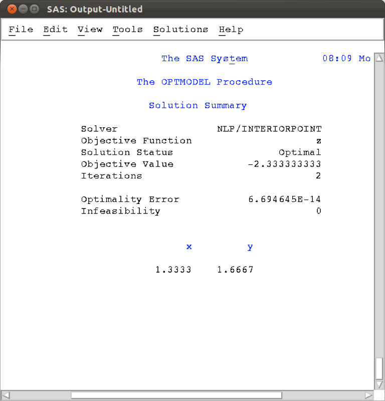
We can also include a domain:
proc optmodel;
var x<=0,y>=2;
min z=x**2-x-2*y-x*y+y**2;
solve;
print x y;
quit;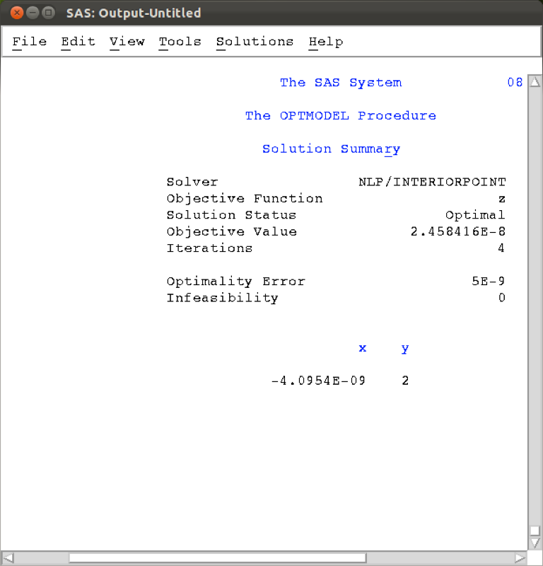
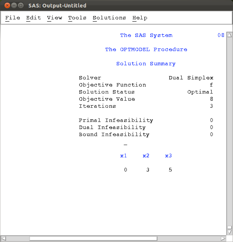
We can solve further more complex optimisation problems, including constraints using the 'constraints' keyword:
proc optmodel;
var x1>=0, x2>=0, x3>=0;
max f=x1+x2+x3;
constraint c1: 3*x1+2*x2-x3<=1;
constraint c2: -2*x1-3*x2+2*x3<=1;
solve;
print x1 x2 x3;
quit;
The output is shown (note the solver used was a variant of simplex).
It is also possible to read in the constraints of a particular optimisation problem from a data set. This can prove to be very handy when dealing with huge problems so it's worth spending time researching that approach.
(Other versions of the above: pdf docx (not recommended))