SAS Chapter 3 - Manipulating Data

3.1 Data steps

A data step is a type of SAS statement that allows you to manipulate SAS data sets. Some of the things we can do include:

1. Copying a data set (with new variables)
2. Concatenating any number of data sets
3. Merging any number of data sets

The following code simply creates a data set in the work library called "j" that is a copy of the data set jjj located in the mat013 library.

data j;
set mat013.jjj;
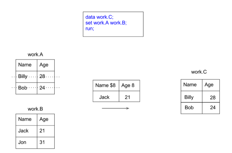
run;

To concatenate two data sets (as shown pictorially) we use the following syntax:

data [New Data Set];
set A B;
run;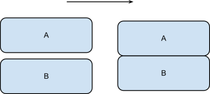

The following code concatenates the jjj and mmm data sets as shown.

data mat013.mmmjjj;
set mat013.mmm mat013.jjj;
run;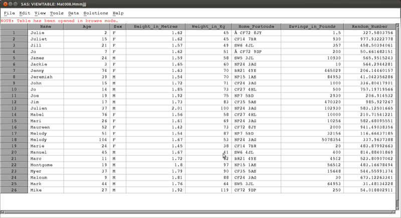

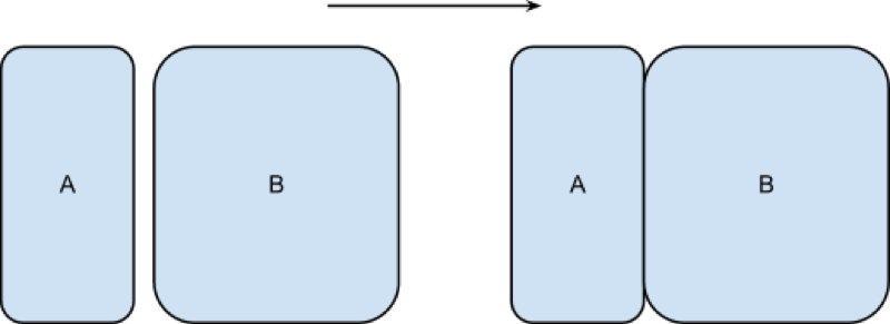
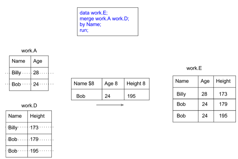
To merge two data sets (as shown pictorially) we use the following syntax:

data [New Data Set];
merge A B;
by [Merge Variable]
run;

Note that the two data sets must be sorted on the merge variable prior to merging.

The following code would merge the two data sets first_data_set and other_data_set in the mat013 library as shown.

proc sort data=mat013.first_data_set;
by name;
run;

proc sort data=mat013.other_data_set;
by name;
run;

data mat013.merged_data_set;
merge mat013.first_data_set mat013.other_data_set;
by name;
run;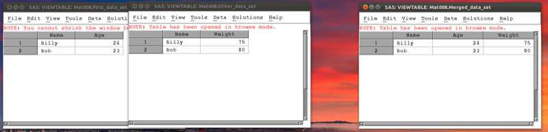

Data steps can be used in conjunction with the where statement to select certain variables. For example consider the data set shown.

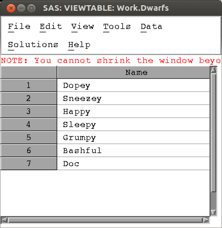
The following code selects only the elements of the above data set that start with a D.

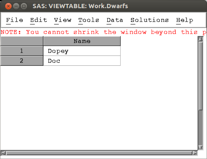
data Dwarfs;
set Dwarfs;
where substr(Name,1,1)="D";
run;

The result is shown in (note that the above code makes use of the substr function that we will see later).

3.2 The program data vector

SAS is able to handle very large data sets because of the way data steps work. In this section we'll explain how it uses the "program data vector" (pdv) to efficiently handle data. The basic steps of compiling a data step are as follows:

1. SAS creates an empty data set.
2. SAS checks the data step for any unrecognized keywords and syntax errors.
3. SAS creates a PDV to store the information for all the variables required from the data step.

4. SAS reads in the data line by line using the PDF.

   (If a "by" statement is used (for example when merging two data sets) the PDF does not empty if there are still observations with the same value of the "by" variable).

5. SAS creates the descriptive portion of the SAS data set (viewable using the "contents" procedure).

An example of how this works with concatenation and an example of how this works with merging is shown.

3.3 Creating new variables

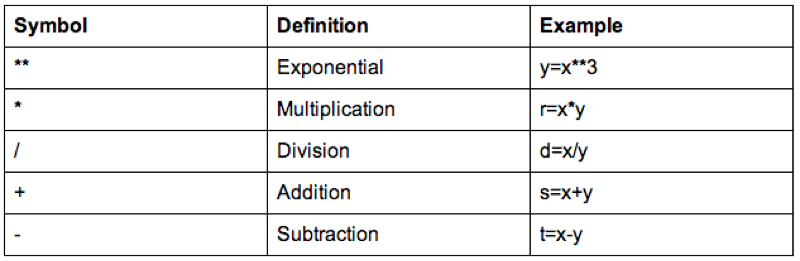
Creating new variables using various arithmetic and/or string relationships is relatively straightforward in SAS. The following code creates a new data set call MMM_with_BMI, with a new variable "BMI" as a function of the height and weight variables in the MMM dataset in the mat013 library.

data mat013.MMM_with_BMI;
set mat013.MMM;
bmi=weight_in_kg/(height_in_metres**2);
run;

Some of the arithmetic functions are shown.

We can also do operations on strings, the following code replaces the variable "Sex" with the first entry of "Sex" (which gets rid of the Male - M and Female - F issue).

data mat013.MMM_with_BMI;
set mat013.MMM;
sex=substr(sex,1,1);
run;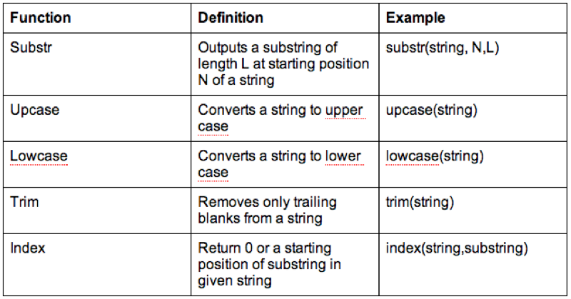

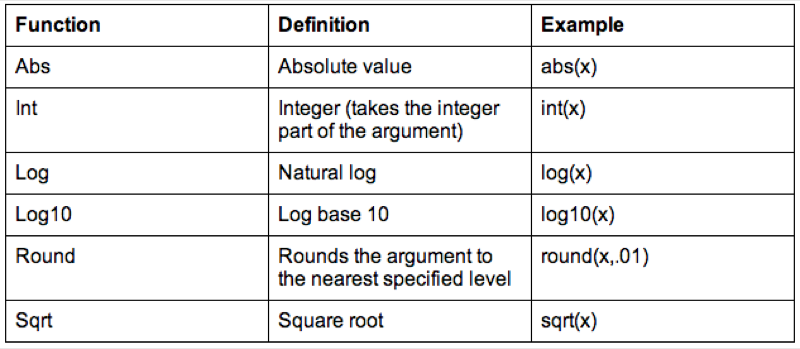
It's worth checking the web for a full list of various SAS functions (there are a huge amount of them).

3.3.1 Dropping and keeping variables.

In this section we'll take a quick look at two simple ways of improving the efficiency of a data step. Recalling how SAS handles a data step (using the pdv as described previously), one immediate way of improving efficiency is to ensure that the pdv only "transports" the variables we require. We do this with the "drop" or "keep" statement.

Let us consider the previous example and assume that we want our MMM_with_BMI data set without the weight and height variables. We use a "drop" statement to get rid of those variables:

data mat013.MMM_with_BMI_nhw(drop=weight_in_kg height_in_metres);
set mat013.MMM;
bmi=weight_in_kg/(height_in_metres**2);
run;

Note that the following code would not give the required output as we are trying to drop the variables from the original data set, however we need those variables to calculate the bmi:

data mat013.MMM_with_BMI_nhw;
set mat013.MMM(drop=weight_in_kg height_in_metres);
bmi=weight_in_kg/(height_in_metres**2);
run;

The keep statement (basically) does the same thing as the drop statement but in reverse, by only keeping the variables we have specified. Which one to use depends simply on whether or not you want to drop or keep more variables.

Note that you cannot use a drop statement and a keep statement in the same data step.

The following code will create a data set with just the bmi variable.

data mat013.just_bmi(keep=bmi);
set mat013.MMM;
bmi=weight_in_kg/(height_in_metres**2);
run;

3.3.2 Renaming variables

The following code creates a data set "JJJ" in the work library which is a copy of the "JJJ" dataset in the mat013 library, renaming the "sex" variable to "gender".

data JJJ(rename=(sex=gender));
set mat013.JJJ;
run;

This can also be used in the set data set:

data JJJ;
set mat013.JJJ(rename=(sex=gender));
run;

3.3.3 Operations across rows

We have seen in previous sections how to create new variables for any given observation (i.e. across columns of a data set). In this section we see how to create variables across rows. Recalling how the program data vector works, this implies that we must find a way to keep certain entries in the pdv for future calculation.

We will demonstrate this using the birthday_money.csv data set as shown.

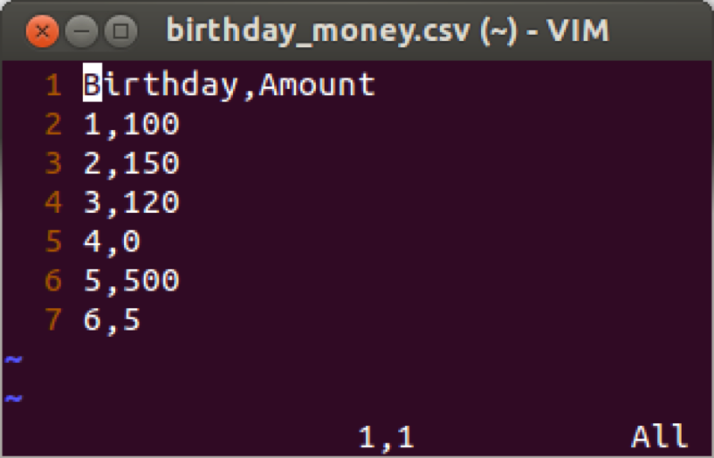
The first such way is to use the "retain" statement. The "retain" statement keeps the last entry for a given variable in the pdv for future calculation. Note that we can give an initial value for a particular variable as shown in the following code (which produces a variable "total" that is a running total of "amount") the output of which is shown.

data bm_analysis;
set mat013.birthday_money;
retain total 0;
total=total+amount;
run;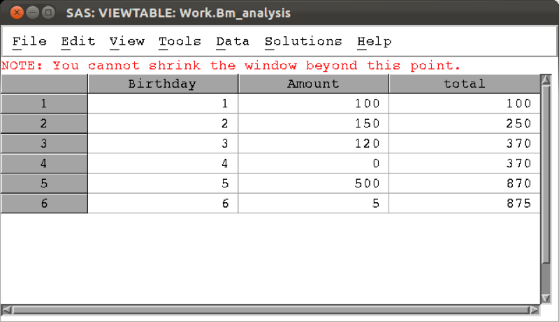

Another tool for such calculations is the "lagn" function which gives the value of a variable from a certain number n of prior steps. The following code gives two new variables, the yearly difference and 2 yearly difference, the result of which is shown.

data bm_analysis;
set mat013.birthday_money;
retain total 0;
total=total+amount;
yearly_diff=amount-lag1(amount);
two_yearly_diff=amount-lag2(amount);
run;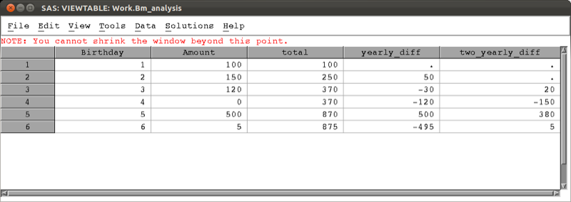

The lag functions can be used in much more complex assignments and in fact when simply wanting to calculate a difference there is a quicker way: using the "difn" function as shown in the code below which gives the same result as shown.

data bm_analysis;
set mat013.birthday_money;
retain total 0;
total=total+amount;
yearly_diff=dif1(amount);
two_yearly_diff=dif2(amount);
run;

3.4 Handling dates

Dates are handled in a particular way in SAS. Let's consider the csv file shown.

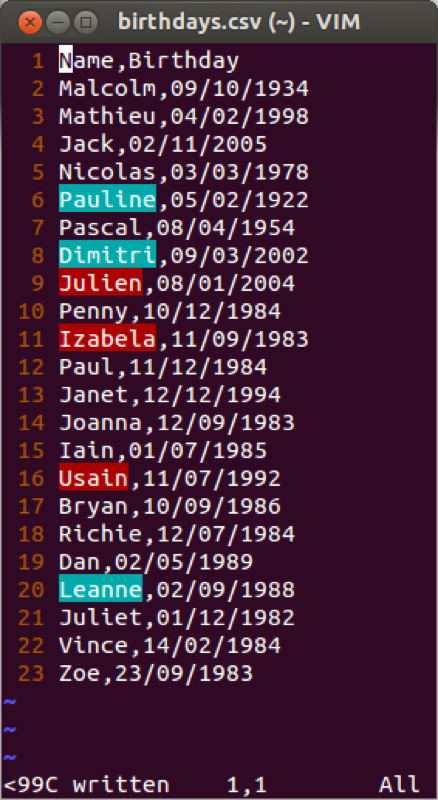
We have seen in Chapter 1 how to import data using proc import. If we use the normal approach an error would occur. This is due to the confusion associated with our birthday variables (the first 20 rows have the date and month values both less than 12). A further option that can be incorporated in proc import is the number of rows that SAS will "pre-read" to identify the type of variables that are to be imported. This is often an easy way to ensure that SAS recognises dates.

proc import datafile='\~birthdays.csv'
out=birthdays
replace;
getnames=yes;
guessingrows=25;
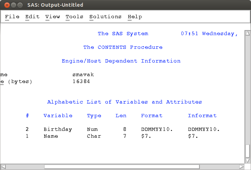
run;

A proc contents run on the above data set shows that the birthday variable data was imported using the informat DDMMYY10. In other words SAS has recognised that the dates were in that particular format.

Another approach is to import files in SAS using a data step and the infile statement. When doing this we can tell SAS the format of the data (whether or not it is a string, numerical or date variables).

data birthdays;
infile '~/birthdays.csv' dlm=',' firstobs=2;
input Name $ Birthday ddmmyy10.;
run;

The infile statement tells SAS where the data is located and the 'dlm' statement tells SAS how the file is delimited (in this case with a comma). The 'firstobs' statement tells SAS where the data starts in the file (in this case the second row as the first row is the name of the variables in our data set). The input statement then allows us to tell SAS the names of the variables as well as the format they are in, here we tell SAS that the second variable is to be called 'Birthday' and it is in the ddmmyy8. format.

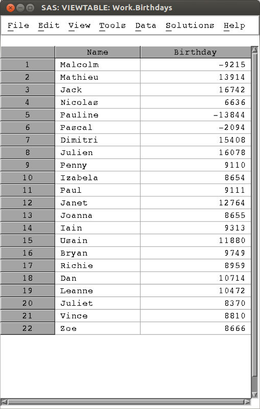
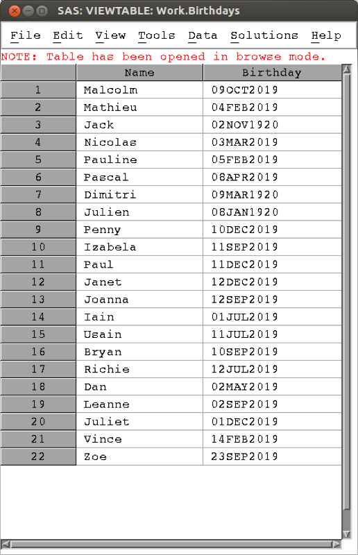
The above output might be a bit confusing, this is due to the fact that SAS handles dates as numbers, using the convention that the 1st of January 1960 is the number 0 (this allows for straightforward arithmetic manipulation of dates). The following code imports the data as above and displays the underlying numeric dates in the date9. format.

data birthdays;
infile '\~/birthdays.csv' dlm=',' firstobs=2;
input Name $ Birthday ddmmyy8.;
format Birthday date9.;
run;

The output is shown. Note that applying the date9. format only changes the appearance of the data.

There are various formats that can be used when importing variables (for dates as well as other variables) and subsequently these same formats can be used to display the data if this is required. Searching online quickly finds other SAS formats.