R Chapter 3 - Manipulating Data
3.1 Vectors and data frames
3.1.1 Vectors
When considering R data frames it is important to recall that they are composed of vectors. Even individual scalars and strings are vectors. This is a very powerful tool.
One important notion when handling vectors is the use of 'recycling'. As all elements are vectors, when performing an operation between two vectors of different length, R automatically repeats (or recycles) the shorter one until it is long enough.
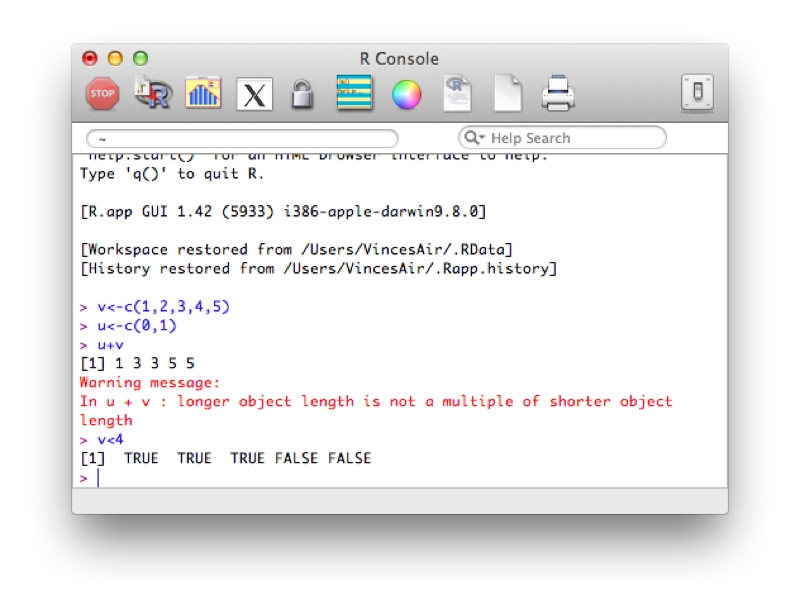
In the previous example, (u+v) we add the elements of both vectors together. R automatically increases the length of u so that the operation becomes (1,2,3,4,5) + (0,1,0,1,0). In the second example we compare the elements of v to 4. R automatically increases the length of the vector containing 4 so that the operation becomes (1,2,3,4,5)<(4,4,4,4,4) which returns a vector of size 5 with boolean (True or False) elements.
This second concept is important when understanding how to select certain variables in R (we saw this briefly in the previous section).
Another important notion in R is that of indexing. We can select elements of a vector by specifying the indices of the elements required:
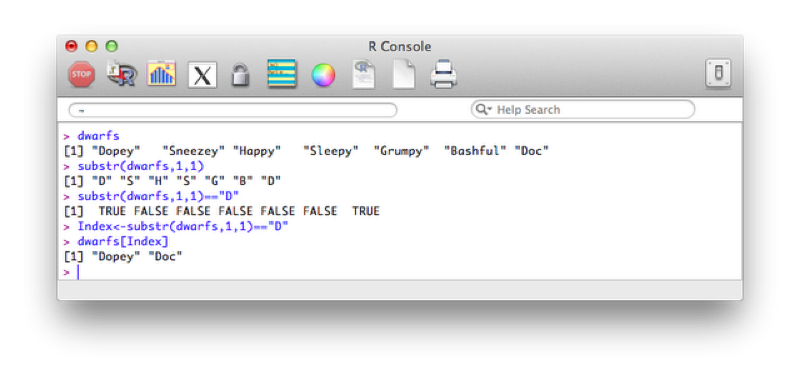
dwarfs<-c("Dopey","Sneezey","Happy","Sleepy","Grumpy","Bashful","Doc")
dwarfs[c(1,4,5)]
dwarfs[3:length(dwarfs)]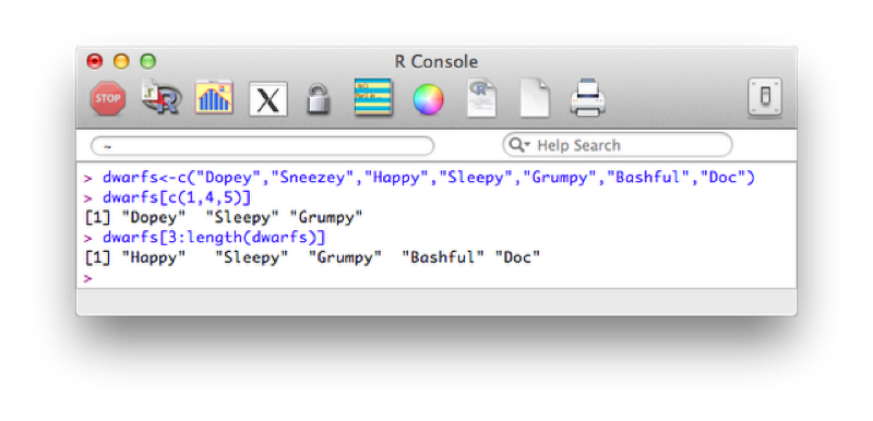
Both of the previous approaches use a vector of indices to indicate the elements we require. The second approach uses a shorthand to create a vector of elements (containing the integers 3 to 5). Another approach is to simply use a vector of boolean values (True or False) to indicate the positions that are to be selected.
Index<-c(TRUE,FALSE,FALSE,FALSE,FALSE,FALSE,TRUE)
dwarfs[Index]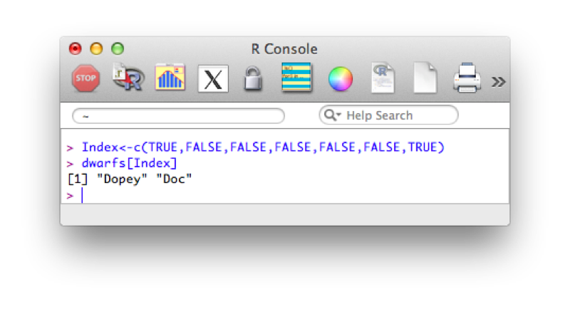
It should be straightforward to realise that we can combine recycling and indexing to filter vectors:
Index<-substr(dwarfs,1,1)=="D"
dwarfs[Index]
The first command creates an index set of boolean variables using the substr function and recycling (in this case used to take the first character of each element). This allows us to obtain the elements of the vector dwarfs with first letter D as shown.
We have seen how to subset vectors using filtering, the same logic applies to data frames.
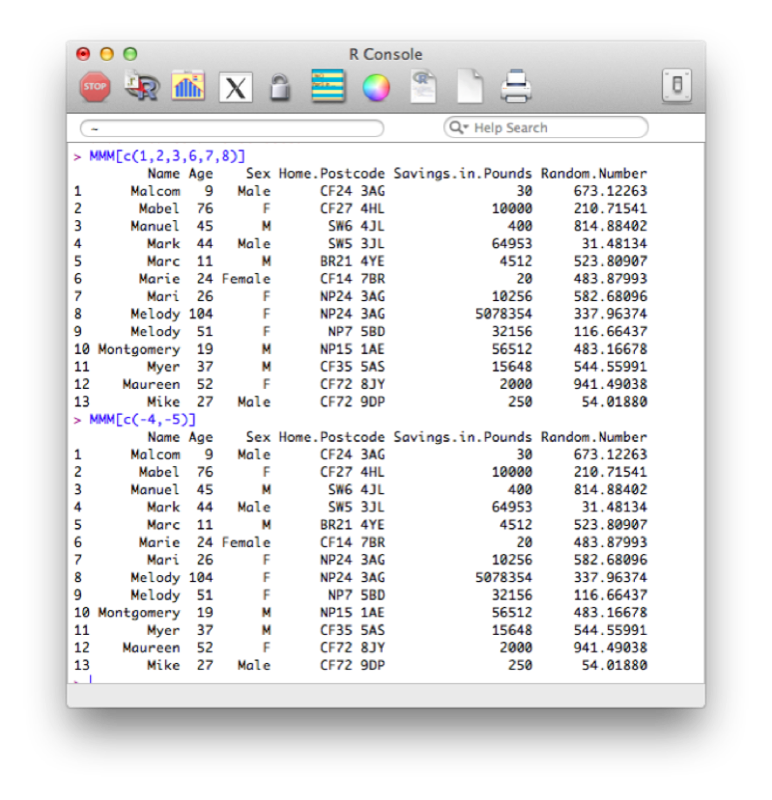
We can first of all use indexing to obtain the variables we want. For example the following code will select the all the variables apart from the 4th and 5th:
MMM[c(1,2,3,6,7,8)]A quicker way is to simply state the variables we want to drop:
MMM[c(-4,-5)]The output of the above code is shown.
We can also list the names of variables we want to keep:
MMM[c("Name","Age","Sex","Home.Postcode","Savings.in.Pounds","Random.Number")]Finally we can create a vector of booleans that gives the same above result or the opposite result (i.e. drops the variables).
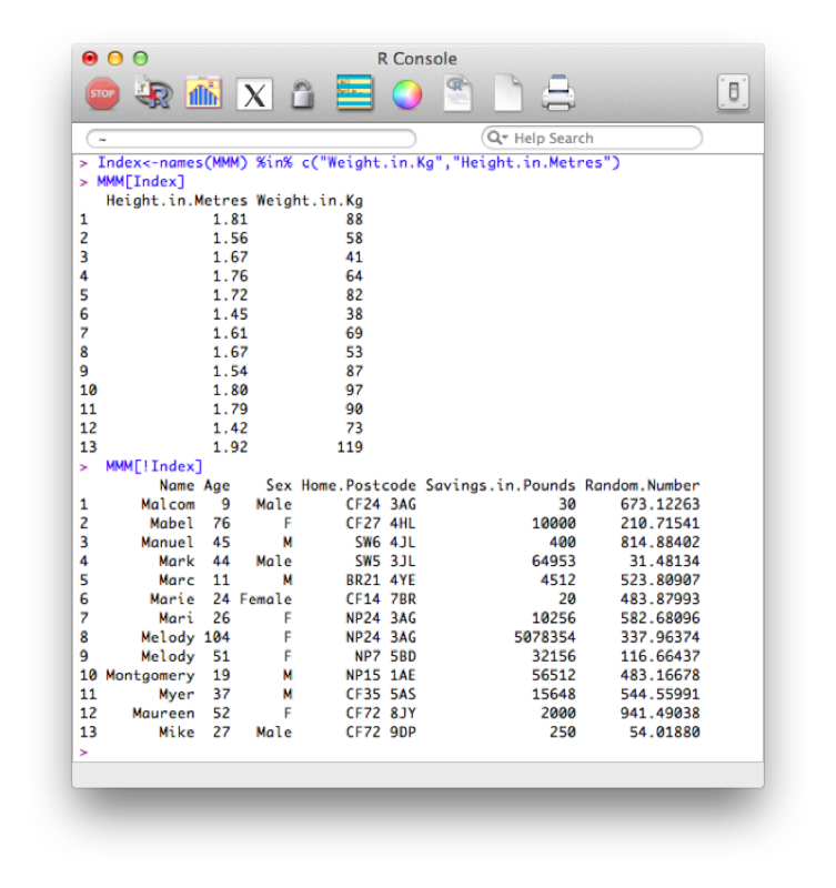
Index<-names(MMM) %in% c("Weight.in.Kg","Height.in.Metres")
MMM[Index]


Index<-names(MMM) %in% c("Weight.in.Kg","Height.in.Metres")
MMM[!Index]
Recall the names function simply gives a vector containing the names of all the variables in the MMM dataset. The %in% operator is used to create a vector of booleans by testing if the elements of names(MMM) are in the vector c("Weight.in.Kg","Height.in.Metres"). The ! operator acting on Index simply negates the booleans contained in Index.
3.1.2 Selecting Observations
We can select any particular element of a data frame in R using the following syntax:
dataframe[i,j]This would give the entry for variable j of observation i as shown.
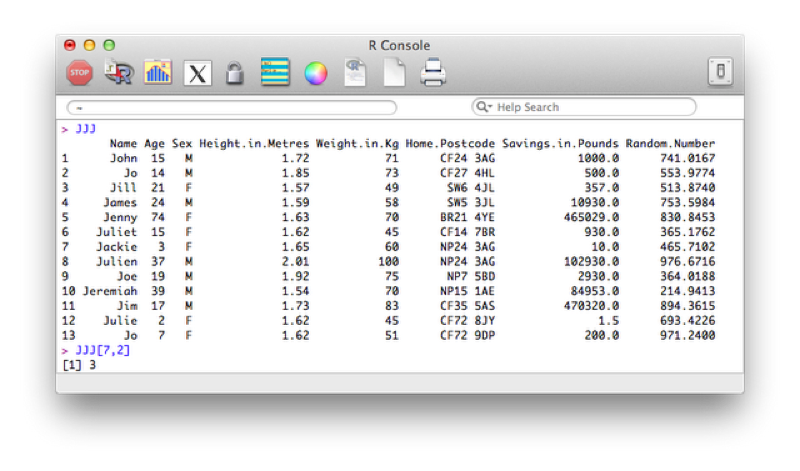
If we ignore one of the indices R simply returns all the entries corresponding to that index. For example the following code would return all the observations for the 7th observation of the JJJ data set:
JJJ[7,]We can also use this to sort a data set. The "order function" returns a set of indices reflecting the ascending order of a vector, thus to sort the JJJ data set by age we use the following code:
JJJ[order(JJJ$Age),]We can use filtering to expand on this and select all observations that obey a particular condition. For example the following code selects entries of JJJ that have age less than or equal to 18:
JJJ[JJJ$Age<=18,]3.2 Merging and concatenating data sets
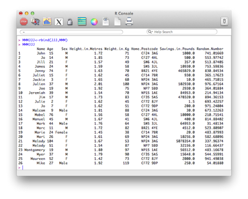
To concatenate two data sets in R we use the rbind function (i.e. we bind the two dataframes by rows).
MMMJJJ<-rbind(JJJ,MMM)Note that both these data sets need to contain all the variables. If one of the datasets does not contain all the variables then you need to add that variable to it and set its values to NA (missing).
To merge two dataframes in R we use the merge function. We'll illustrate this with the following data set:
Name<-c("Bob","Ben")
Weight<-c(75,94)
other_data_set<-data.frame(Name,Weight)
We'll merge this new data set with the data set we created in Chapter 1.
merged_data_set<-merge(first_data_set,other_data_set,"Name")(or equivalently:)
merged_data_set<-merge(x=first_data_set,y=other_data_set,by="Name")The output is shown.
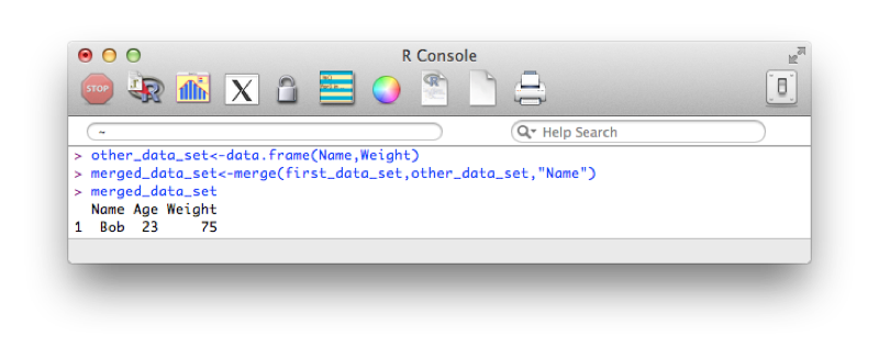
Note that the merge statement only selects observations that are present in both files. We can pass further arguments to the merge statement that allow us to select all the values from a particular data set and/or both data sets. These operations are at times called 'joins' (and are very common in SQL which we shall see in Chapter 5). The basic merge statement (as above) would be referred to as an 'inner' join.
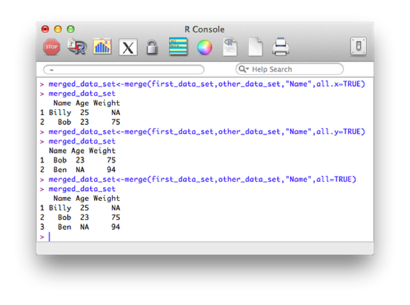
A left outer join (selecting all variables from the first data set):
merged_data_set<-merge(first_data_set,other_data_set,"Name",all.x=TRUE)A right outer join:
merged_data_set<-merge(first_data_set,other_data_set,"Name",all.y=TRUE)A full outer join:
merged_data_set<-merge(first_data_set,other_data_set,"Name",all=TRUE)The output of the above is shown.
3.3 Creating new variables
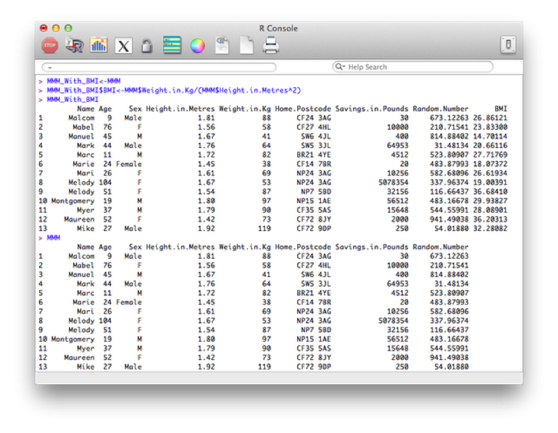
Creating new variables using various arithmetic and/or string relationships is straightforward in R. The following code creates a new data set call MMM_with_BMI as a copy of the MMM data set and then adds a new variable "BMI" as a function of the height and weight variables in the MMM_with_BMI dataset.
MMM_With_BMI<-MMM
MMM_With_BMI$BMI<-MMM$Weight.in.Kg/(MMM$Height.in.Metres^2)
MMM_With_BMI
The output is shown.
The above code is quite long though, so we can use the within function which is similar to the with function. It lets R know you are working within a particular data frame.
MMM_With_BMI <- within(MMM, BMI <- Weight.in.Kg/(Height.in.Metres^2))The output is shown:

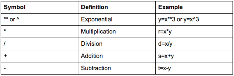
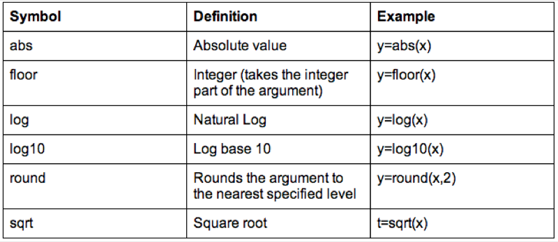
Some of the arithmetic functions available in R are shown.
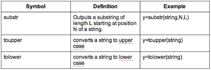
We can also do operations on strings, the following code replaces the variable Sex with the first character of Sex (which gets rid of the Male - M and Female - F issue).
MMM_With_BMI$Sex<-substr(MMM_With_BMI$Sex,1,1)Some examples of string functions are shown.
It's also worth checking the web for other R functions (there is a huge amount of them).
3.3.1 Renaming variables
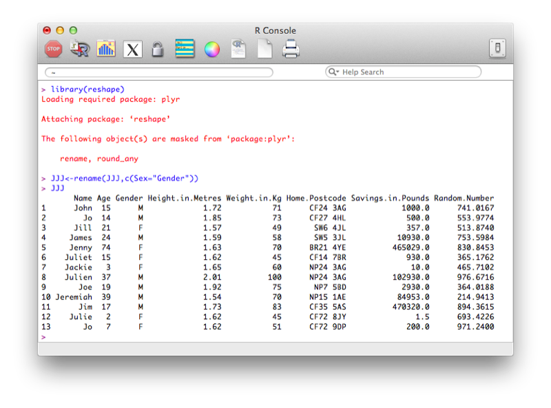
To rename variables one can use the rename function from the reshape library (that can be installed as we have seen in previous section).
library(reshape)
JJJ<-rename(JJJ,c(Sex="Gender"))
The output is shown.
Another option is to use the "fix" function that opens the dataset in a GUI that easily allows for modification of the dataset (including the name of the variables). Note that changes are saved on close of the fix environment.
fix(JJJ)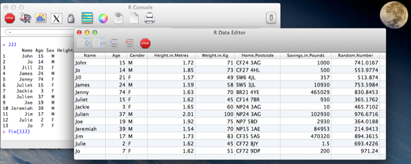
3.3.2 Operations across rows
As discussed previously, the columns of a data frame can be manipulated very easily as they are just vectors. In the next section we will see how to manipulate vectors using flow control statements but we will take a quick look at two functions that allow for quick and easy manipulation across rows.
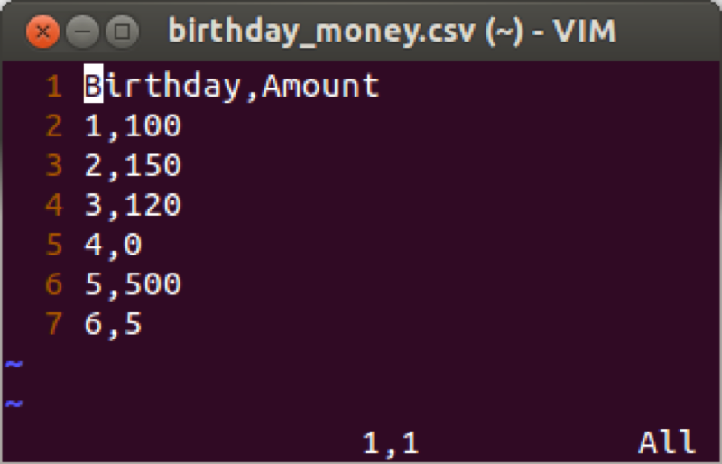
We will demonstrate this using the birthday_money.csv data set as shown.
Suppose we want to take a cumulative sum of the birthday money, we create a new variable call total using the cumsum function that returns the cumulative sum of elements of a vector.
birthday_money$total<-cumsum(birthday_money$Amount)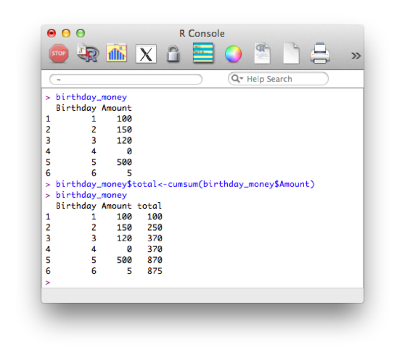
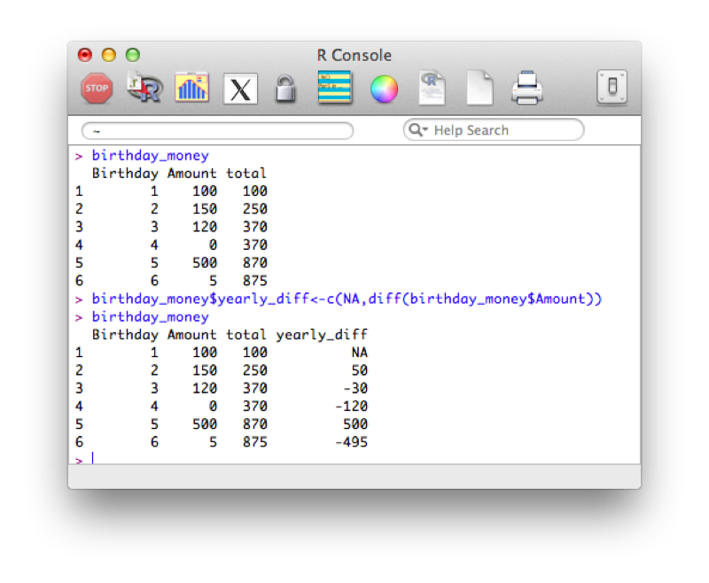
Another similar tool is to use the "diff" function that calculates consecutive differences of elements of a vector:
birthday_money$yearly_diff<-c(NA,diff(birthday_money$Amount))Note that we also include a first entry of our column "yearly_diff" as "NA", this is because the output of diff will be shorter than the length of the original vector.
3.4 Handling dates in R
Dates are a particular class in R. When importing dates, they are imported as strings.
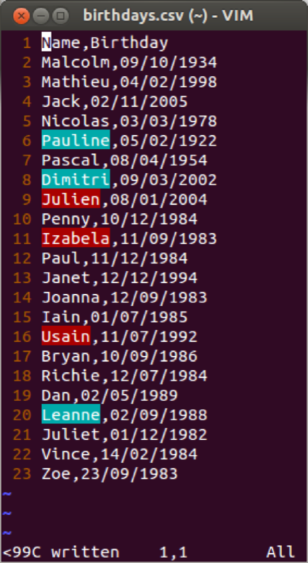
We import the file and create a data frame in the usual way:
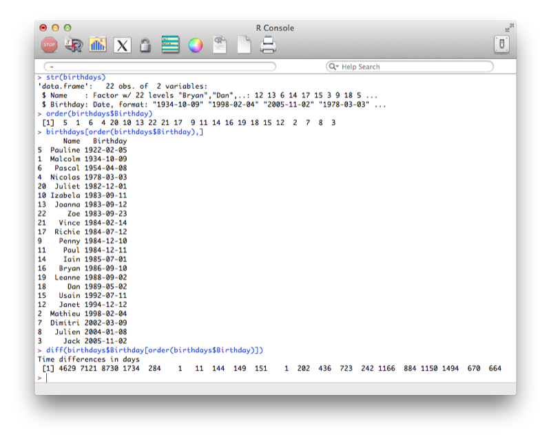
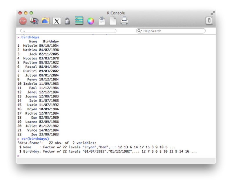
birthdays<-read.csv("~/birthdays.csv")Using the "str" command to view the structure of our data frame:
str(birthdays)The output is shown confirming that the dates are recognized as strings (recall that by default read.csv imports strings as factors).
In this current format if we tried to carry out any mathematical manipulation of the dates we would not succeed. We can however tell R that certain variables are dates. We do this using the "as.dates" function by describing the format our dates are in:
birthdays$Birthday<-as.Date(birthdays$Birthday,"%d/%m/%Y")The format is indicated using "%x" where "x" can be of various formats as show.
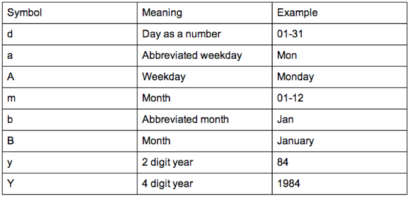
We'll now check the structure of our data frame, re-order (using the order function - that returns the indices of the elements of a vector in order) our birthdays and calculate the difference between birthdays (using the diff function).
str(birthdays$Birthday)
order(birthdays$Birthday)
sorted<- birthdays[order(birthdays$Birthday),]
diff(birthdays$Birthday[order(birthdays$Birthday)])
The output of all this is shown.