R Chapter 2 - Basic Statistical Procedures
2.1 Procedures
In the previous chapter we were introduced to some very basic aspects of R:
- what R looks like
- how to import data into R
- how to export data into R
In this chapter we will take a closer look at procedures that allow us to analyse and manipulate data. Vectors are the building blocks of all R objects. Single numeric/string variables are in fact vector of size 1. Almost all procedures in R are obtained by applying functions to vectors. Details as to how R handles these operations will be explained in the next chapter (so don't worry about it too much for now).
The procedures we are going to look at in this chapter are:
- Viewing datasets
- Summarising the contents of data sets
- Obtaining summary statistics of data sets
- Obtaining frequency tables
- Obtaining linear models
- Plotting data
2.2 A list of procedures
2.2.1 Utility procedures
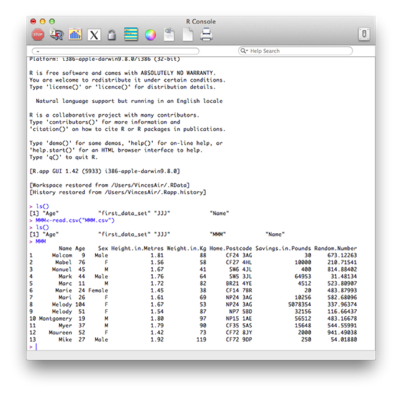
We have seen how to view and entire data set (by simply printing the name of the object in question).
We illustrate this once again by considering the MMM data set shown, (imported using read.csv).
At times we might not want to open the data set but simply gain some information as to what is in the data set.
To view only the names of the variables of our data set we use the name function as shown.
names(MMM)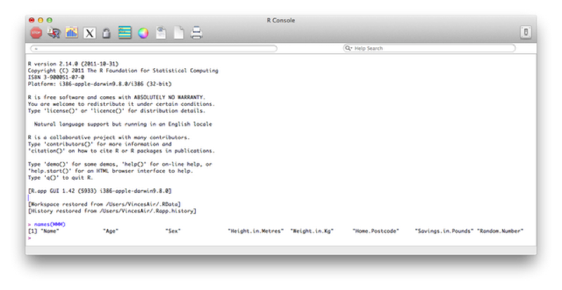
If we had a very large data set then we could quickly view the first/last few entries using the head/tail function as shown.
head(MMM)
tail(MMM)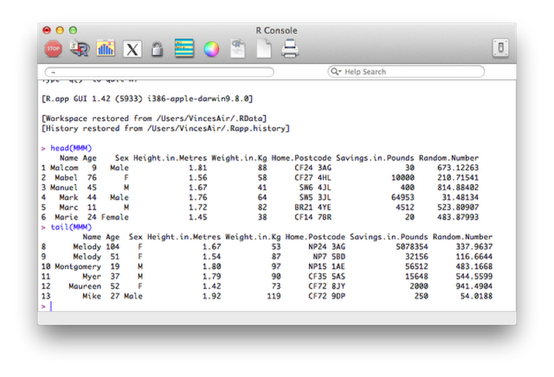
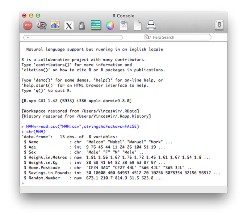
Finally if we would like to view a description of the overall structure of a data set we can use the str function as shown.
str(MMM)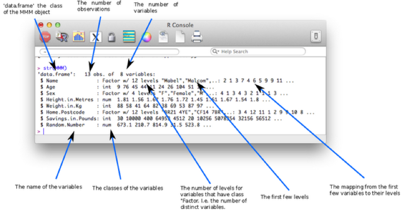
The class of the imported character variables are Factors, this is due to the importation method (read.csv) automatically converting the character variables in this form - details about "Factors" are given below. The reason this occurs is the default value of stringsAsFactors (used in the read.csv function) is TRUE, the following code forces the characters retain their class without conversion.
MMM<-read.csv("MMM.csv",stringsAsFactors=FALSE)The factor stores the nominal values as a vector of integers in the range [ 1... k ] (where k is the number of unique values in the nominal variable), and an internal vector of character strings (the original values) mapped to these integers. This is often a much more efficient way of handling strings.
2.2.2 Descriptive statistics
To gain an initial set of summary statistics of a data frame we can use the summary function:
summary(MMM)The output of which is shown.
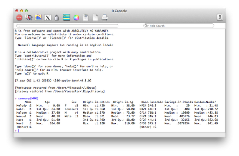
Recall that most "things" in R are objects and "summary" is a good example of a generic function that works on most objects. If you are faced with a new object (for example the output of a regression analysis) it is sometimes worth trying to apply summary on it to get some initial information.
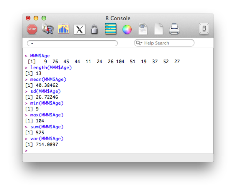
To obtain a particular summary statistic of a specific variable, we can use functions that apply to vectors and select the vectors from the dataset.
To select a particular column (as a vector) from our dataset, we use the following command:
MMM$AgeWe can then apply various functions to this vector:
length(MMM$Age)
mean(MMM$Age)
sd(MMM$Age)
min(MMM$Age)
max(MMM$Age)
sum(MMM$Age)
var(MMM$Age)
The output of which is shown.
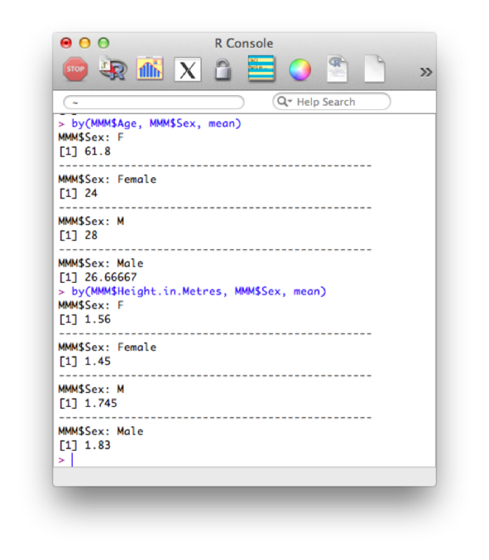
We can compartmentalise our results using the by function. The general syntax for the by function is given below:
by(data=dataFrame , Indices=grouping variables, FUN= a function)We'll use this to obtain the mean age and height compartmentalised by sex:
by(MMM$Age, MMM$Sex, mean)
by(MMM$Height.in.Metres, MMM$Sex, mean)
The output of which is shown.
The above code subsets the data frame by the grouping variable. If we want to just carry out an action on a vector (as above, we're only actually interested in the Age vector or the Height vector) then we can also use the "tapply function". This applies a function to a vector according to the levels of another vector:
tapply(MMM$Age, MMM$Sex, mean)Finally, to reduce the number of keystrokes, we can use the with statement. This tells R to evaluate everything within a given data frame. The following code reproduces the above results:
with(data=MMM,by(Age,Sex,mean) )
with(data=MMM,tapply(Age, Sex, mean))
Note: the data= statement can be omitted.
2.2.3 Frequency Tables
The table function allows us to obtain frequency tables of data sets. As an example let us consider the data set shown. The table function creates a "table" (a particular type of R object):
table(math_tests$Teacher,math_tests$Pass.Fail)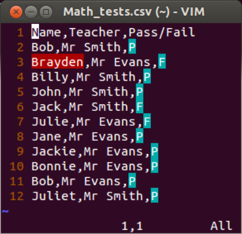
Again we can write this as:
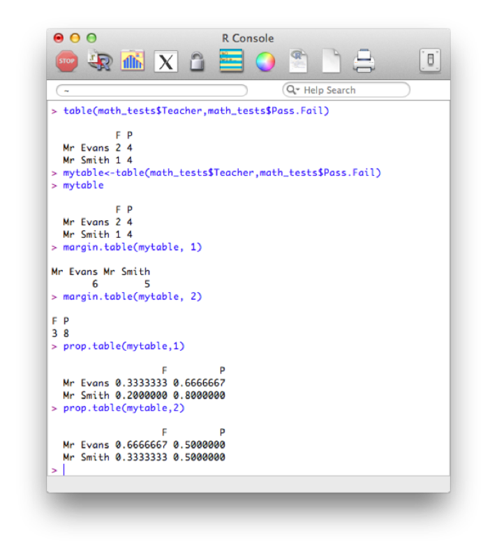
with(math_tests,table(Teacher,Pass.Fail))We can save this table as a new object and use the prop command to gain row and column totals and proportions:
mytable<-table(math_tests$Teacher,math_tests$Pass.Fail)
margin.table(mytable, 1)
margin.table(mytable, 2)
prop.table(mytable,1)
prop.table(mytable,2)
The output of all this is shown.
2.2.4 Correlations
The following lines of code select only the columns from MMM that are numeric. An explanation of this will follow in the next chapter.
MMM[,sapply(MMM,is.numeric)]The correlation 'cor' function only acts upon numeric vectors (and/or dataframes), hence the selection of solely numeric values first.
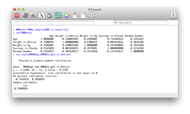
MMMnum<-MMM[,sapply(MMM,is.numeric)]
cor(MMMnum)
The cor function however does not give tests of significance. We can obtain significance tests between two variables using cor.test:
cor.test(MMM$Age,MMM$Height.in.Metres)The output is shown.
As is often the case in open source software, packages are independently developed and need to be called to be used in R. Above we have shown the very basic approach to obtaining correlations in R, we will now use the rcorr function from the Hmisc package.
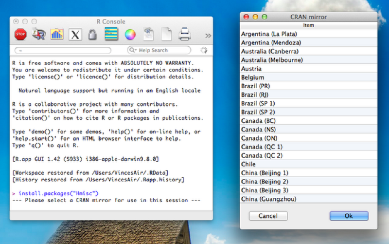
To install the package we use the following code:
install.packages("Hmisc")Once that happens a window opens asking us to choose the mirror from which to download. This is shown.
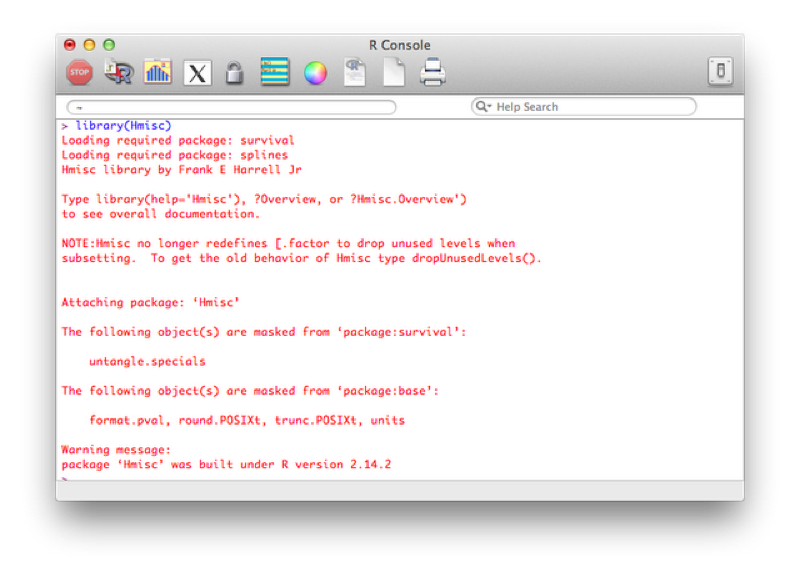
Once that is done to load the package the following code is required:
library(Hmisc)or:
require(Hmisc)To see the packages currently loaded we can use the following code:
search()Note: Packages can also be installed by selecting the 'Packages' tab and selecting the package required for installation.
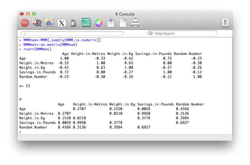
Using this package, we will use the rcorr function that gives the correlation matrix for a data set. Note that the data set must be numeric and in matrix form. The following code selects the numeric variables from the MMM data set and converts the result to a matrix:
MMMnum<-MMM[,sapply(MMM,is.numeric)]
MMMmat<-as.matrix(MMMnum)
Once this is done we can get the correlation matrix using the following code:
rcorr(MMMmat)The output is shown.
2.2.5 Linear Models
In this section we very briefly see the syntax for some basic linear models in R.
The general syntax for linear regression is as follows in R:
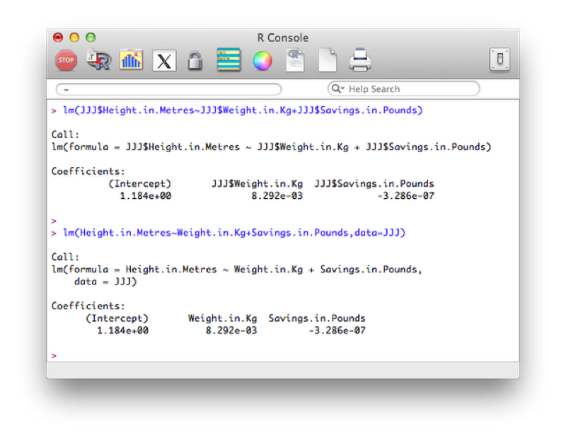
lm(outcome~predictors)The following code will be used to investigate whether or not there is a linear model of height with weight and savings and predictors (in two ways, the second is slightly more compact and leaves less room for confusion):
lm(JJJ$Height.in.Metres~JJJ$Weight.in.Kg+JJJ$Savings.in.Pounds)
lm(Height.in.Metres~Weight.in.Kg+Savings.in.Pounds,data=JJJ)
The results are shown.
To get the full set of results from the regression analysis we use the following code:
summary(lm(Height.in.Metres~Weight.in.Kg+Savings.in.Pounds,data=JJJ))The output is shown.
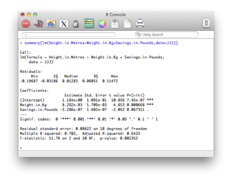
Looking at the p value we see that the overall model should not be rejected, however the detailed results show that perhaps we could remove savings from the model.
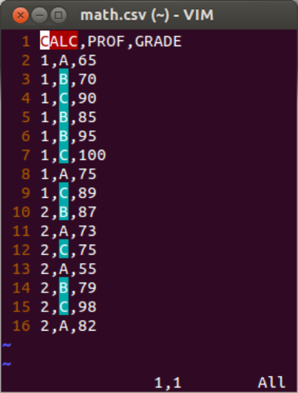
Analysis of variance (ANOVA) can be done easily in R. We shall show this using a new data set (math.csv) shown.
aov(outcome~class,data)
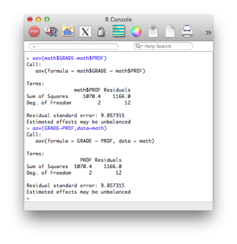
We will use the "aov" function to see if the grades obtained by students depend on their teacher (in two ways, the second is slightly more compact):
aov(math$GRADE~math$PROF)
aov(GRADE~PROF,data=math)
The results are shown.
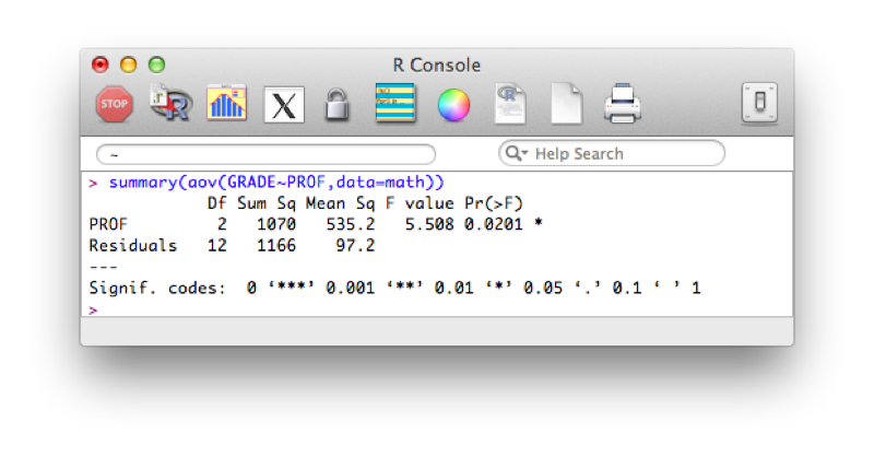
To get the full set of results from the ANOVA we use the following code:
summary(aov(GRADE~PROF,data=math))The results are shown.
2.2.6 Plots and charts
Note that due to the object oriented nature of R, almost all of the above outputs have a "plot" attribute.
The simplest way to produce a histogram in R is to use the "hist" function. The following code gives a histogram for the height of entries in the JJJ data set as shown.
hist(JJJ$Height.in.Metres)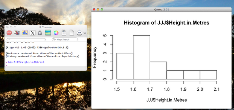
The simplest way to produce a scatter plot in R is to use the "plot" function. The following code gives a scatter plot for the height against weight of entries in the JJJ data set as shown.
plot(JJJ$Weight.in.Kg,JJJ$Height.in.Metres)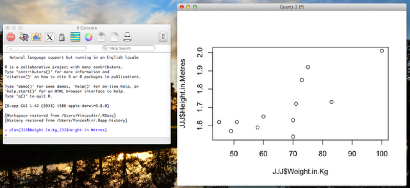
There are various other ways to obtain similar graphs, as well as change the look and feel of our graphs. We won't go into this here but you are encouraged to look into it (in particular the ggplot package is widely used).
2.3 Exporting output
All the non graphical outputs from R are objects, as such they can be output to a file (to be copied into another document if need be) using the write statements of Sections 1.4. However to export graphical output, we use any of the following statements (depending on the output format required):
pdf("mygraph.pdf")
win.metafile("mygraph.wmf")
png("mygraph.png")
jpeg("mygraph.jpg")
bmp("mygraph.bmp")
postscript("mygraph.ps")
Once that command is written we use a normal R command to create a plot and finally we close the output file with the following statement:
dev.off( )The following code creates a png file entitled "height_v_weight_plot" with the previous scatter plot.
png("height_v_weight_plot.png")
plot(JJJ$Weight.in.Kg,JJJ$Height.in.Metres)
dev.off( )