R Chapter 1 - Introduction
1.1 The Environment
R can be run in a number of different modes, for the purpose of this course we will be focusing on 'interactive mode' through the graphical user interface (GUI); 'batch mode' is also available but will not be covered here. Note that the screenshots and accompanying screencasts for this course were produced with R version 2.14 running on Mac OSX The look and feel on other operating systems will differ slightly.
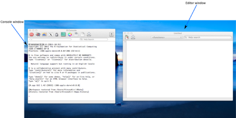
The visible windows are:
- The editor window
- The console
We can write commands directly into the console window or we can create a script file and edit it in the editor window, highlighting specific text we wish to run. The second approach has the benefit of being able to save the commands written in the script files, although it takes more time (and in fact the commands we write directly in the console can also be saved to a file).
When writing scripts it is good practice to include comments in our files that help describe what the code does. The way to do this in R is with the # symbol before text. The following code is ignored by R:
#2+2Using the highlight + run approach is akin to copying and pasting the text in the interpreter but R scripts can also be run directly (so that they can be run on servers or as routines without the need to have a user interact).
1.2 Objects
R is an extremely versatile programming language. In particular R is an "object oriented language". The significance of this is that everything (functions, data files, outputs of a regression analysis) is an "object". The type of object is called the "class" and what one can do to a class is called a "method". The advantage of this is that when a new "class" is developed one simply needs to ensure that is has relevant "methods", to be compatible with other objects.
As an example, various objects in R have a "plot" method, for example the output of a regression analysis can be plotted using the same command as one would use to plot a scatter plot of a data set.
R has a wide range of data types (which are themselves objects). The 2 classes corresponding to data sets we will concentrate on in this course are:
- Vectors
- Data frames
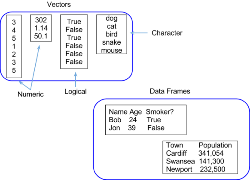
Vectors are simply collections of variables of a particular type ("Numeric", "Character", "Boolean" etc). In R a type of variable is called a "mode", representing how it is stored in the computer memory. Data frames are collections of vectors and correspond to data sets. Technically, data frames are lists with dimensions, which are themselves just generic vectors. One might say a collection of equal length vectors (thus allowing the rectangular shape). Some examples of vectors and data frames are shown.
Let's import some data!
1.3 Importing Data
We will consider two approaches to importing data:
- Direct input
- Importing an external data set (xls, csv etc...)
In practice you will never use the direct input method but let's take a look for completeness (although it is very useful when wanting to quickly test a few things). This will also give us our first experience of the editor window!
Let us create a data set named first_data_set which will include the following data:
    Name, Age
    Bob, 23
    Billy, 25
To do so write the following code in the editor window:
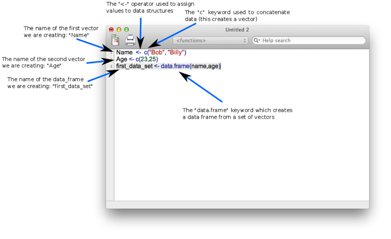
Name <- c("Bob","Billy")
Age <- c(23,25)
first_data_set <- data.frame(Name,Age)
Let's take a look at the shown screenshot of this. You may notice that some elements of the text are highlighted, this is to emphasise key words (note that this doesn't happen automatically on Windows).
- The first two lines of code make use of the
<-operator that assigns an object to a variable. - The objects in questions are created using the
c(ombine) function that creates a vector. We use this to create 2 vectors: Name and Age. - Finally we put the 2 vectors into a data frame using the
data.framecommand.
We run this code by highlighting it and pressing ctrl + 'r' (cmd + enter on Mac). Note that when we submit code this way it also appears in the console window. We could have in fact directly type this code into the console window. For those familiar with command line commands the console works in a very similar way. We can press the up arrow repeatedly to cycle through previous commands and use tab to autocomplete.
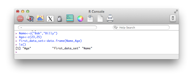
The data set first_data_set is now saved to memory. To view all the data structures in memory we use the simple line of code:
ls()A screenshot of the output is shown. We see that there are actually 3 objects in memory, the two vectors (Name and Age) as well as the data frame (first_data_set).
To view our data set, we simply type the name (as shown):
first_data_set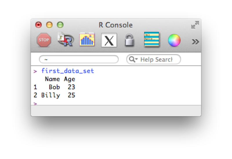
Using direct input is of course not at all realistic when trying to import larger data sets.
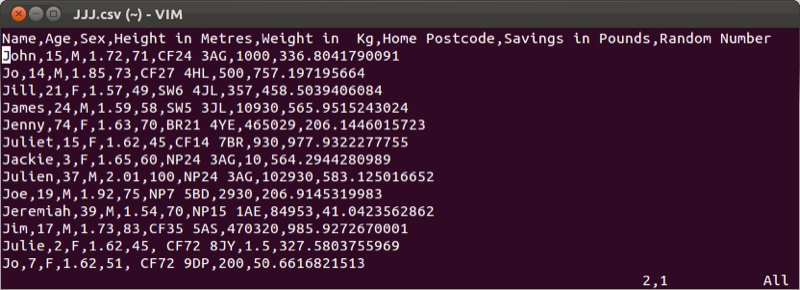
Often large data sets will be saved in comma-separated values (csv) format which can be read by most (all?) software. We will import the data set shown (here viewed in a simple text editor).
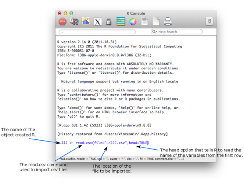
We will import this data set into R using the following code:
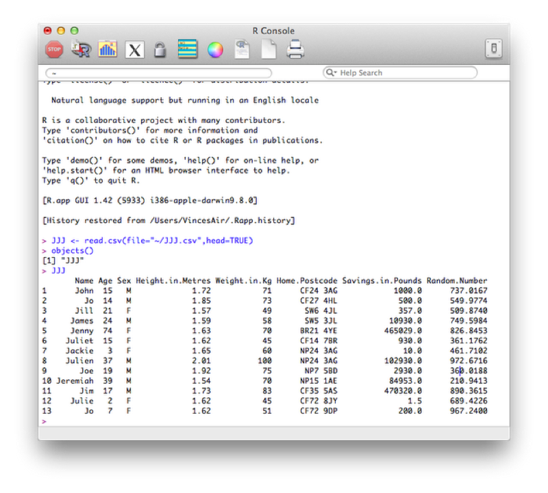
JJJ <- read.csv(file="~/JJJ.csv",head=TRUE)Let's take a look at the screenshot shown. Note here that we are not using the text editor but directly writing code in the console (this is often how I prefer to use R for short bits of code).
read.csv- is the command which is used to tell R to read in data from a csv file.file- an option tells R where the csv file is located.head- an option tells R to read the variable names from the first row of the csv file. Note that this command can be omitted (the default value isTRUE).
We have omitted other options (such as sep which can be used to change the default separator from , to something else).
Running the code (by either pressing enter if using the console or highlighting and running as before is using the editor) gives the required object as shown.
In the following chapters we will learn how to create new data sets from old data sets and as such it may become necessary to export files to csv.
1.4 Exporting Data Sets
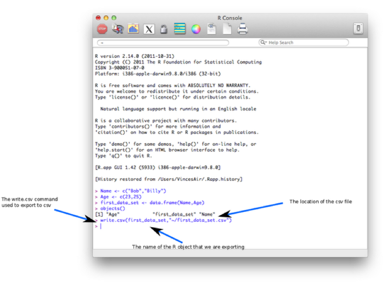
We will export our first data set (first_dataset) to csv using the following line of code:
write.csv(first_data_set,"~/Desktop/first_data_set.csv")Let's take a look at the screenshot.
write.csvis the command which is used to tell R to read in data from a csv file.- The first command tells R which R object to export.
- The second command tells R the location of the csv file.