Calculating the expected wait in a tandem queue with blocking using Sage

In this post I’ll describe a particular mathematical model that I’ve been working on for the purpose of a research paper. This is actually part of some work that I’ve done with +James Campbell an undergraduate who worked with me over the Summer.

Consider the system shown in the picture below:

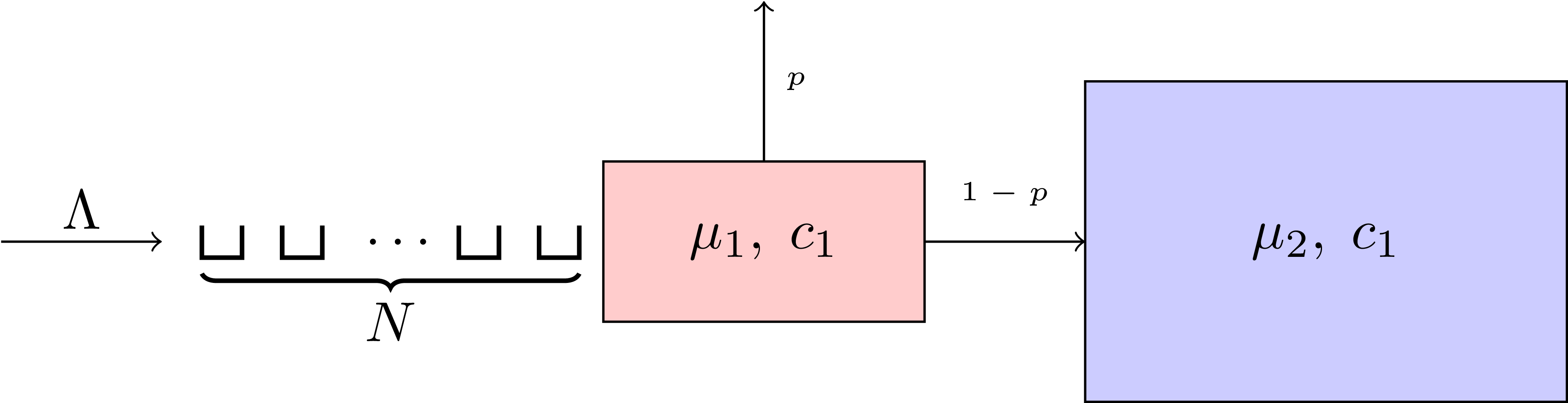
This is a system composed of ‘two queues in tandem’ each with a number of servers $c$ and a service rate $\mu$. It is assumed here (as is often the case in queueing theory) that the service rate is exponentially distributed (in effect that the service time is random with mean $1/\mu$).

Individuals arrive at the queue with mean arrival rate $\Lambda$ (once again exponentially distributed).

There is room for up to $N$ individuals to wait for a free server at the first station. After their service at the first station is complete, individuals leave the system with probability $p$, but if they don’t and there is no free place in the next station (ie there are not less than $c_2$ individuals in the second service center) then they become blocked.

There are a vast array of applications of queueing systems like the above (in particular in the paper we’re working on we’re using it to model a healthcare system).

In this post I’ll describe how to use Markov chains to be able to describe the system and in particular how to get the expected wait for an arrival at the queue.

I have discussed Markov chains before (mainly posts on my old blog) and so I won’t go in to too much detail about the underlying theory (I think this is perhaps a slightly technical post so it is mainly aimed at people familiar with queueing theory but by all means ask in the comments if I can clarify anything).

The state space

One has to think about this carefully as it’s important to keep track not only of where individuals are but whether or not they are blocked. Based on that one might think of using a 3 dimensional state space: $(i,j,k)$ where $i$ would denote the number of people at the first station, $j$ the number at the second and $k$ the number at the first who are blocked. This wouldn’t be a terrible idea but we can actually do things in a slightly neater and more compact way:

$S = \left\{(i,j)\in\mathbb{Z}^{2}_{\geq 0}\;|\;0\leq j \leq c_1+c_2,\; 0\leq i\leq c_1+N-\max(j-c_2,0)\right\}$

In the above $i$ denotes the number of individuals in service or waiting for service at the first station and $j$ denotes the number of individuals in service at the second station or blocked at the first station.

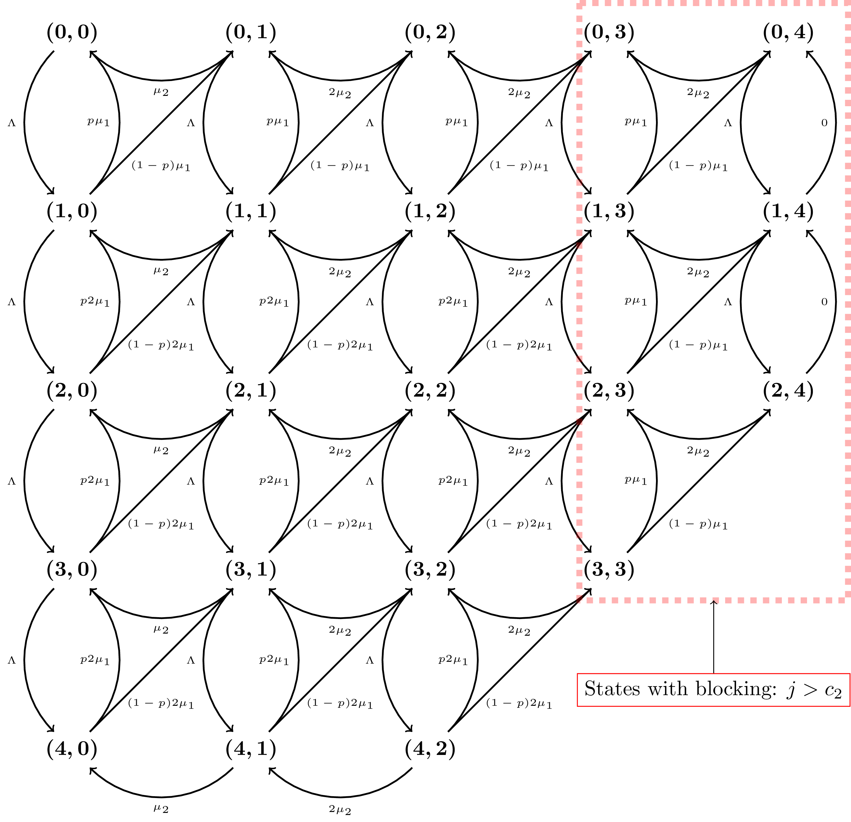
The continuous time transition rates between two states $(i_1,j_1)$ and $(i_2, j_2)$ are given by:

$q_{(i_1,j_1), (i_2,j_2)}= \begin{cases} \Lambda, & \text{ if } \delta = (1,0)\\ \min(c_1-\max(j_1-c_2,0),i_1)(1-p)\mu_1, & \text{ if } \delta = (-1,1)\\ \min(c_1-\max(j_1-c_2,0),i_1)p\mu_1, & \text{ if } \delta = (-1,0)\\ \min(c_2, j_1)\mu_2, & \text{ if } \delta = (0,-1) \end{cases}$

where $\delta=(i_2,j_2)-(i_1,j_1)$.

Here’s a picture of the Markov Chain for $N=c_1=c_2=2$:

The steady state probabilities

Using the above we can index our states and keep all the information in a matrix $Q$, to obtain the steady state distributions of the chain (the probabilities of finding the queue in a given state) we then simply solve the following equation:

$\pi Q = 0$

subject to $\sum \pi = 1$.

Here’s how we can do this using Sage:

    class Tandem_Queue():
        """
        A class for an instance of the tandem_queue
        """
        def __init__(self, c_1, N, c_2, Lambda, mu_1, mu_2, p):
            self.c_1 = c_1
            self.c_2 = c_2
            self.N = N
            self.Lambda = Lambda
            self.mu_1 = mu_1
            self.mu_2 = mu_2
            self.p = p
            self.m = c_1 + c_2 + 1
            self.n = c_2 + 1
            self.state_space = [(i, j)  for j in range(c_1 + c_2 + 1) for i in range(self.c_1 + self.N - max(j - self.c_2, 0) + 1)]
            if p == 1:  # Reduces state space in particular case of p = 1
                self.state_space = [state for state in self.state_space if state[1] == 0]
            Q = [[self.q(state1, state2) for state2 in self.state_space] for state1 in self.state_space]
            for i in range(len(Q)):
                Q[i][i] = - sum(Q[i])
            self.Q = matrix(QQ, Q)
            self.expected_wait_cache = {}

        def q(self, state1, state2):
            """
            Returns the rate of transition between to given states.
            """
            delta = list(vector(state2) - vector(state1))
            if delta == [1, 0]:
                return self.Lambda
            if delta == [-1, 1]:
                return min(self.c_1 - max(state1[1] - self.c_2, 0), state1[0]) * self.mu_1 * (1 - self.p)
            if delta == [-1, 0]:
                return min(self.c_1 - max(state1[1] - self.c_2, 0), state1[0]) * self.mu_1 * self.p
            if delta == [0, -1]:
                return min(state1[1], self.c_2) * self.mu_2
            return 0

        def pi(self):
            """
            Solves linear system.
            """
            A = transpose(self.Q).stack(vector([1 for state in self.state_space]))
            return A.solve_right(vector([0 for state in self.state_space] + [1]))

Most of the above is glorified book keeping but here’s a quick example showing what the above does and how it can be used. First let’s create an instance of our problem with $N=c_1=c_2=2$, $5\mu_2=2p=\mu_1=1$ and $\Lambda=5$.

sage: small_example = tandem_queue(2,2,2,5,1,1/5,1/2)
sage: small_example.Q
22 x 22 dense matrix over Rational Field (use the '.str()' method to see the entries)

We see that if we return $Q$ we get a 22 by 22 matrix which if you recall the picture above corresponds to the 22 states in that picture.

We can see the states by just typing:

sage: small_example.state_space
[(0, 0),
 (1, 0),
 (2, 0),
 (3, 0),
 (4, 0),
 (0, 1),
 (1, 1),
 (2, 1),
 (3, 1),
 (4, 1),
 (0, 2),
 (1, 2),
 (2, 2),
 (3, 2),
 (4, 2),
 (0, 3),
 (1, 3),
 (2, 3),
 (3, 3),
 (0, 4),
 (1, 4),
 (2, 4)]

If you check carefully they all correspond to the states of the picture above.

Now what we would like to know is the probability of being in any given state. To do this we need to solve the matrix equation $\pi Q = 0$ such that $\sum \pi=1$.

This is done in Sage (for any matrix Q) using the following:

sage: A = transpose(Q).stack(vector([1 for state in self.state_space]))
sage: A.solve_right(vector([0 for state in self.state_space] + [1]))

There we build a matrix A with an added column of 1s and then solve the corresponding equation using solve_right (note that we transposed the matrix). If you look at the class definition this was all defined earlier so we can in fact just run:

sage: small_example.pi()
(974420487508335328592/55207801002325145206717477, 6717141852060739142960/55207801002325145206717477, 25263720112088475982400/55207801002325145206717477, 107693117265184715581000/55207801002325145206717477, 499825193288571759140000/55207801002325145206717477, 7567657557556535357400/55207801002325145206717477, 50835142813671411162000/55207801002325145206717477, 177836071295654602905000/55207801002325145206717477, 638540135036394350075000/55207801002325145206717477, 2305924001256099701875000/55207801002325145206717477, 26439192416069771765000/55207801002325145206717477, 185599515623092483825000/55207801002325145206717477, 700026867396942548625000/55207801002325145206717477, 2256398553097737112500000/55207801002325145206717477, 4700830318953618984375000/55207801002325145206717477, 61385774570987050093750/55207801002325145206717477, 444444998037114715312500/55207801002325145206717477, 3393156381219452445312500/55207801002325145206717477, 15476151589322058007812500/55207801002325145206717477, 41152314633066177343750/55207801002325145206717477, 352285141439825390625000/55207801002325145206717477, 1826827211896183837890625/4246753923255780400516729)

That’s not super helpful displayed like that (all the arithmetic is being done exactly) so here’s a quick plot of the probabilities:

sage: p = list_plot(small_example.pi(), axes_labels = ['State', 'Probability'])
sage: p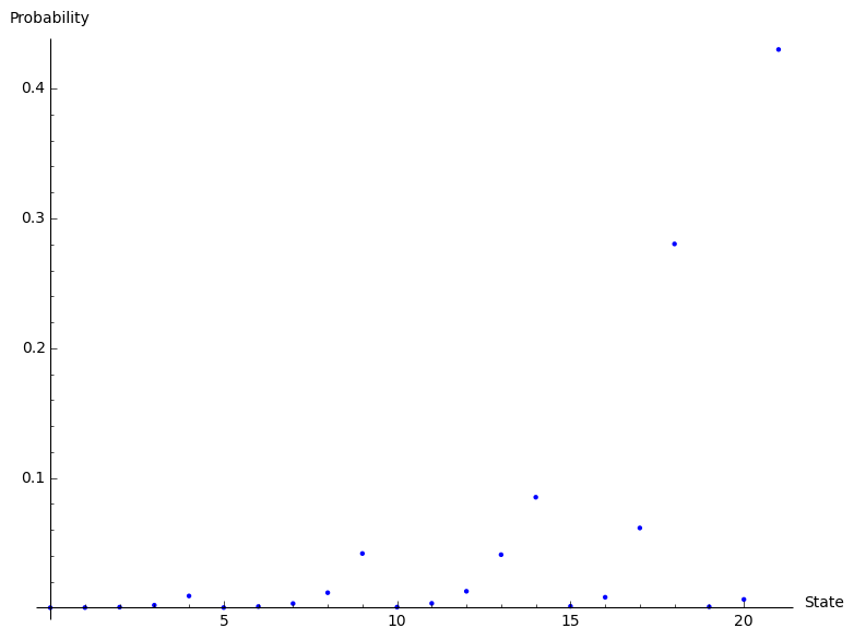

That plot could be made a lot prettier an informative (by for example using the names of the states as xticks) but it will do for now. We can see from there for example that the most probable state of our queue (with the parameters we picked) is to be in the last state (see list above) which is $(2,4)$.

Out of interest here’s a plot when we change $\Lambda=1/2$ (a tenth of what we did above):

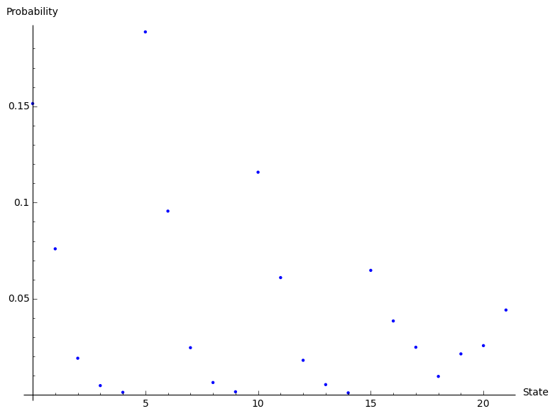
We see that now the most probable state is the sixth state (Python/Sage indexing starts at 0), which corresponds to $(0,1)$.

Here’s an animated plot of the steady state distribution for a larger system as $\Lambda$ increases, displayed in a more informative way (the two dimensions corresponding to $i$ and $j$):

All of that is very nice and interesting but where things get very useful is when trying to calculate the mean time one would expect to wait in a queue.

Mean expected wait in the queue

If we consider all states $(i,j)\in S$ only a subset of them will actually imply a wait:

If there are less than $c_1$ individuals in the first station then anyone who arrives has direct access to a server;
If there are more than $N+c_1$ individuals in the first station then anyone who arrives will be lost to the system.

With a little bit of thought (recalling what the $i$s and $j$s represent) we see that the states that incur a wait are given by:

$S_A=\{(i,j)\in S\;|\; i + \max(j - c_2,0)< c_1 + N \}$

Now if we know the expected wait when arriving in any state $(i,j) \in S_A$ we can get the mean wait as:

$w = \frac{\sum_{(i,j)\in S_A}w(i,j)\pi_{(i,j)}}{\sum_{i + \max(j - c_2, 0) < c_1 + N}\pi_{(i,j)}}$

where $w(i,j)$ denotes the expected time spent in any given state $(i,j)$. We are in essence, summing over arrivals that will have a wait and dividing by the probability of an individual not being lost to the system, which happens when $i + \max(j - c_2, 0) < c_1 + N$.

Obtaining $c(i,j)$ is relatively simple. We consider the ‘almost’ same Markov chain as above (except that we ignore arrivals). In this instance a jump from one step to another will only occur if a service occurs at the first station (with rate $\min(c_1-\max(j-c_2,0),i)\mu_1$) or if a service at the second station (with rate $\min(c_2, j)\mu_2$).

So the mean time spent in state $(i,j)$ is the inverse of the total exit rate:

$c(i,j)=\frac{1}{\min(c_2,j)\mu_2+\min(c_1-\max(j-c_2,0),i)\mu_1}$

Using that notion we are in effect discretizing the ‘ignore arrivals’ Markov chain. Once a transition occurs we can obtain the probability of where the service occurs:

The probability of the service being at the first station:

$p_{s_1}=p_{s_1}(i,j)=\frac{\min(c_1-\max(j-c_2,0),i)\mu_1}{\min(c_1-\max(j-c_2,0),i)\mu_1 + \min(c_2,j)\mu_2}$

The probability of the service being at the second station:

$p_{s_2}=p_{s_2}(i,j)=\frac{\min(c_2,j)\mu_2}{\min(c_1-\max(j-c_2,0),i)\mu_1 + \min(c_2,j)\mu_2}$

We can use all of the above to put together a nice recursive formula for the expected wait $w(i,j)$ in terms of the expected wait of states that are in effect getting closer and closer to having no wait:

$w(i,j) = \begin{cases} 0,&\text{ if }(i,j)\in A\\ c(i,j) + p_{s_2}w(i,j-1)+p_{s_1}(pw(i-1,j)+(1-p)w(i-1,j+1)), &\text{ otherwise} \end{cases}$

where $A$, is the set of states with no wait: $i+\max(j-c_2,0) < c_1$

Using the recursive formula is actually very easy to implement in code (we use a dictionary to cache calculated values to not make sure we don’t waste any time).

Here is a reduced version of the methods that need to be added to above to get this to work in Sage (you need to add self.expected_wait_cache = {} to the __init__ method):

    def _pi_dict(self):
        """
        Obtain a dictionary which indexes the states.
        """
        self.pi_list = self.pi()
        return {state:self.pi_list[index] for index, state in enumerate(self.state_space)}

    def p_service_1(self, state):
        """
        Returns the discretized probability of a service occurring at first station
        """
        if self.p == 1:
            return 1
        return min(self.c_1 - max(state[1]- self.c_2, 0), state[0]) * self.mu_1 / (min(self.c_1 - max(state[1]- self.c_2, 0), state[0]) * self.mu_1 + min(self.c_2, state[1]) * self.mu_2)

    def p_service_2(self, state):
        """
        Returns the discretized probability of a service occurring at second station
        """
        if self.p == 1:
            return 0
        return  min(self.c_2, state[1]) * self.mu_2 / (min(self.c_1 - max(state[1]- self.c_2, 0), state[0]) * self.mu_1 + min(self.c_2, state[1]) * self.mu_2)

    def mean_time_in_state(self, state):
        """
        Returns the mean time in any given state before a transition occurs
        """
        return  1 / (min(self.c_1 - max(state[1]- self.c_2, 0), state[0]) * self.mu_1 + min(self.c_2, state[1]) * self.mu_2)

    def expected_wait(self, state):
        """
        Function that returns the expected time till absorption for a given state
        """
        if state in self.expected_wait_cache:
            return self.expected_wait_cache[state]
        if state not in self.state_space:  # If state outside of boundary. (Might not need this after new conditions below)
            return 0
        if state[0] + max(state[1] - self.c_2, 0) < self.c_1:  # If absorbing state
            self.expected_wait_cache[state] = 0
            return 0
        self.expected_wait_cache[state] =  (self.mean_time_in_state(state) + self.p * self.p_service_1(state) * self.expected_wait((state[0] - 1, state[1])))
        if (state[0] - 1, state[1] + 1) in self.state_space:
            self.expected_wait_cache[state] += (1-self.p) * self.p_service_1(state) * self.expected_wait((state[0] - 1, state[1] + 1))
        if (state[0], state[1] - 1) in self.state_space:
            self.expected_wait_cache[state] += self.p_service_2(state) * self.expected_wait((state[0], state[1] - 1))
        return self.expected_wait_cache[state]

    def mean_expected_wait(self):
        """
        Returns the mean wait
        """
        self.pi_dict = self._pi_dict()
        accepting_states = [state for state in [s for s in self.state_space if s[0] + max(s[1] - self.c_2, 0) < self.c_1 + self.N]]
        prob_of_accepting = sum([self.pi_dict[state] for state in accepting_states])
        return sum([self.expected_wait(state) * self.pi_dict[state] for state in accepting_states]) / prob_of_accepting

Using all of the above we can get the expected wait for our system:

sage: small_example = Tandem_Queue(2,2,2,1/2,1,1/5,1/2)
sage: small_example.mean_expected_wait()
60279471210745371/50645610005072978
sage: n(_)
1.19022105182873

Below is a plot showing the effect on the mean wait as demand increases in the plot below for a large system:

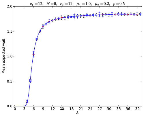
What that plot shows is the calculated values (solid blue) line going through box plots of the simulated value. Perhaps in another blog post some day I’ll write about how to simulate the above but I think that’s probability sufficient for now.

If it’s of interest all of the above code can be downloaded here or at this gist.