Chapter 18 - Connection between optimal and Nash flows

Recap

In the previous chapter:

We defined routing games;
We defined and calculated optimal flows;
We defined and calculated Nash flows.

In this Chapter we’ll look at the connection between Optimal and Nash flows.

Potential function

Definition of a potential flow

Given a routing game $(G,r,c)$ we define the potential function of a flow as:

$\Phi(f)=\sum_{e\in E}\int_0^{f_e}c_e(x)dx$

$A routing game.\label{L17-img04}$

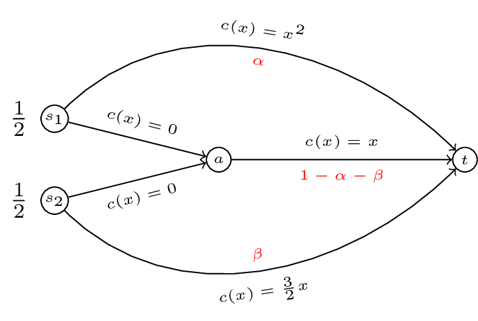
Thus for the routing game shown we have:

$\Phi((\alpha,\beta))=\frac{\alpha^3}{3}+\frac{3\beta^2}{4}+\frac{(1-\alpha-\beta)^2}{2}$

A plot of $\Phi(\alpha,\beta)$ is shown.

$$\Phi(\alpha,\beta)$.\label{L18-plot01}$

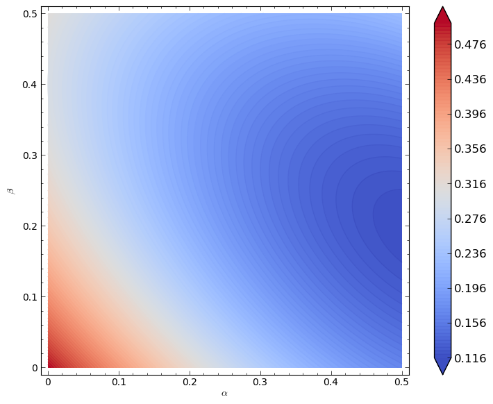
We can verify analytically (as before) that the minimum of this function is given by $(\alpha,\beta)=(1/2,1/5)$. This leads to the following powerful result.

Theorem connecting the Nash flow to the optimal flow

A feasible flow $\tilde f$ is a Nash flow for the routing game $(G,r,c)$ if and only if it is a minima for $\Phi(f)$.

This is a very powerful result that allows us to obtain Nash flows using minimisation techniques.

It also points towards a connection between Nash flows and optimal flows.

Marginal costs

Definition of marginal cost

If $c$ is a differentiable cost function then we define the marginal cost function $c^*$ as:

$c^*=\frac{d}{dx}(xc(x)$

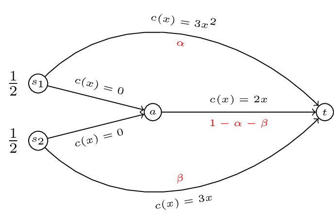
For our running example we have the marginal cost functions given.

$$(G,r,c)$.\label{L18-img01}$

We now state our last theorem of the course:

Theorem connecting optimal flows to Nash flows

A feasible flow $f^*$ is an optimal flow for $(G,r,c)$ if and only if $f^*$ is a Nash flow for $(G,r,c^*)$.

Using this we can compute the optimal flow for our original game by computing the Nash flow for our modified game.

If we assume that both players use both paths then we have:

$\begin{aligned} 3\alpha^2&=2(1-\alpha-\beta)\\ 3\beta&=2(1-\alpha-\beta) \end{aligned}$

This gives $\beta=\frac{2}{5}(1-\alpha)$ implying $3\alpha^2=\frac{6}{5}(1-\alpha)$ which gives (as before) $f^* \approx(.4633,0.2147)$.

We will finish the course by looking at an interesting example that occurs in routing game theory.

Braess’s Paradox

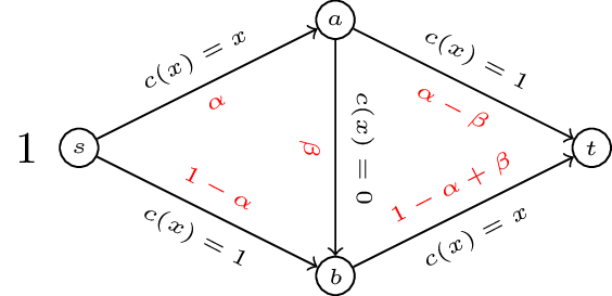
Consider the routing game shown.

$A simple routing game.\ref{L18-img02}$

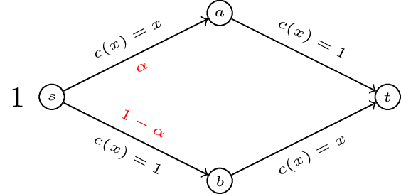
If we write down the potential function $\Phi(\alpha)=\alpha^2/2+(1-\alpha)^2/2+(1-\alpha)+\alpha=\alpha^2 -\alpha + 3/2$. The flow $\tilde f=1/2$ minimises the potential function and so is a Nash flow. In fact for this example we have $\tilde f=f^*$ and $C(\tilde f)=C(f^*)=3/2$.

If we modify the network by adding capacity to our network with another edge of zero cost.

$Brass's Paradox. \label{L18-img03}$

We can compute the potential function and optimise but we can quickly verify that $\tilde f=(\alpha,\beta)=(1,1)$ is a Nash flow by comparing with other potential paths. Thus we have $C(\tilde f)=2$. By adding an edge to our network with a very “cheap” latency cost the situation has been made worse!