SAS Chapter 2 - Basic Statistical Procedures
2.1 Procedures
In the previous chapter we were introduced to some very basic aspects of SAS:
- what SAS looks like
- how to import data into SAS
- how to export data from SAS
In this chapter we will take a closer look at "procedure steps" which allow us to call a SAS procedure to analyse or process a SAS dataset. In the previous chapter we have already seen two procedure steps:
- proc import
- proc export
The procedures we are going to look at in this chapter are:
- Viewing datasets
- Summarising the contents of data sets
- Obtaining summary statistics of data sets
- Obtaining frequency tables
- Obtaining linear models
- Plotting data
The general syntax for these procedures in SAS is given below:
proc [NAME OF PROCEDURE] data=[NAME OF SAS DATA SET];
[Options for Procedure being used]
run;
Some of the options that can be used in a procedure step include:
- "var" - which tells SAS which variables are to be processed.
- "by" - which tells SAS to compartementalize the procedure for each different value of the named variable(s). The data set must first be sorted by those variables.
- "where" - select only those observations for which the expression is true.
2.2 A list of procedures
2.2.1 Utility procedures
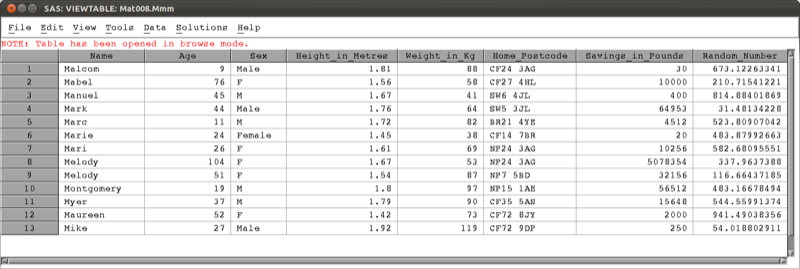
We have already seen that we can open and view a data set by simply double clicking on the data set in the explorer window. A data set can also be viewed by using the "print" procedure.
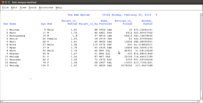
We'll do this by considering the MMM data file shown (imported using an import procedure).
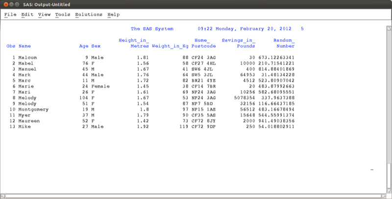
The following code will run the "print" procedure:
proc print data=mat013.mmm;
run;
which outputs the data set to the output window as shown.
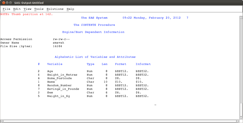
At times we might not want to open the data set but simply gain some information as to what is in the data set. This is equivalent to checking the label on a present without unwrapping it. We do this using the "contents" procedure.
proc contents data=mat013.mmm;
run;
This outputs summary information as shown.
A procedure that will be needed, when using more complex procedures and larger data sets, is the "sort" procedure.
proc sort data=mat013.mmm;
by age;
run;
Note that this procedure makes use of the "by" statement which tells SAS which variable to sort our observations on (in this case the variable age). Recall that the data set is not sorted. If we run the above "sort" procedure, at first nothing seems to happen, however if we view the data set again (using proc print or otherwise) we see (as shown) that the data set is now sorted.
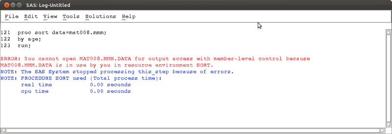
Important: If you have the mat013.mmm data set open in browser mode (i.e. having double clicked on the data set in the explorer window) when running the "sort" procedure, checking your log shows you an error as shown. Always close any browser windows when processing a data set - or use the "print" procedure!
### Descriptive statistics
In this section we will go over some of the procedures needed to obtain descriptive statistics.
The first procedure we consider is the "means" procedure. We can use the following code to obtain various summary statistics relating to the age variables of the mat013.mmm dataset.
proc means data=mat013.mmm;
var age;
run;
We can specify the particular summary statistics we want (if none are specified a default set is displayed).
proc means data=mat013.mmm N mean std min max sum var css uss;
var age;
run;
We can also choose to display the summary statistics for more than one variable
proc means data=mat013.mmm N mean std min max sum var css uss;
var age height_in_metres;
run;
We can compartmentalise our data results using the "by" statement. Note that the data set must be sorted on the same variable.
proc means data=mat013.mmm N mean std min max sum var css uss;
var age height_in_metres;
by sex;
run;
Another way of compartmentalising results is using the "class" statement. This is very similar to the "by" statement and does not require the prior sorting of your data set.
proc means data=mat013.mmm N mean std min max sum var css uss;
var age height_in_metres;
class sex;
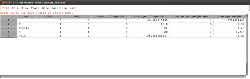
run;Finally, it's also possible to create a data set from the "means" procedure.
proc means data=mat013.mmm N mean;
var age height_in_metres;
class sex;
output out=summary_of_mmm
N(age)=number_of_age_obs
mean(age)=average_of_age_obs
N(height_in_metres)=number_of_height_obs
mean(height_in_metres)=average_height;
run;
The above code creates a data set called "summary_of_mmm" in the work library (the default library if no library is specified) with two variables "number_of_obs" and "average_of_obs" which give the number and mean for the observations as calculated by the "means" procedure as shown.
The "univariate" procedure allows for the calculation of univariate statistics in SAS. The following code will output all the default univariate statistics for all the variables.
proc univariate data=mat013.mmm;
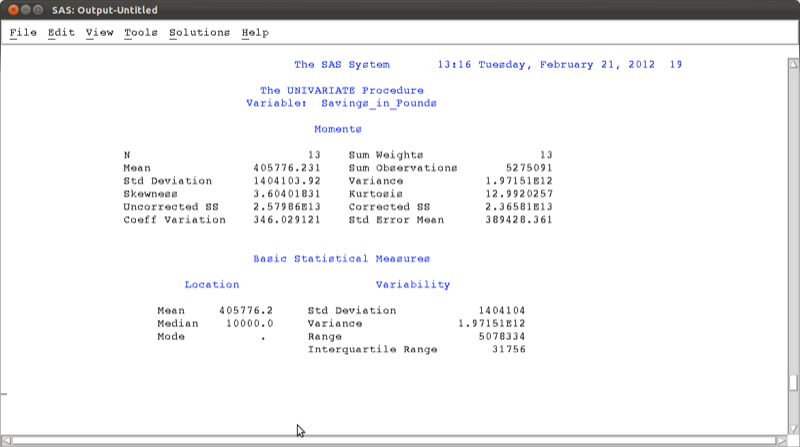
run;We can choose to run the "univariate" procedure on a subset of the variables, using the "var" statement.
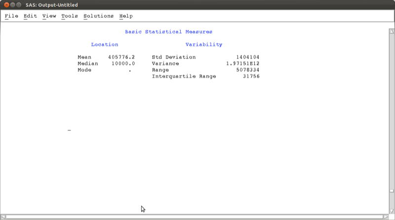
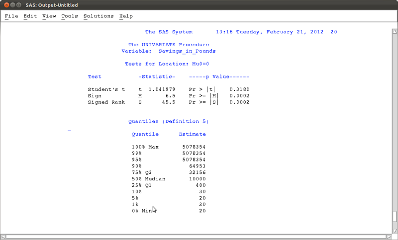
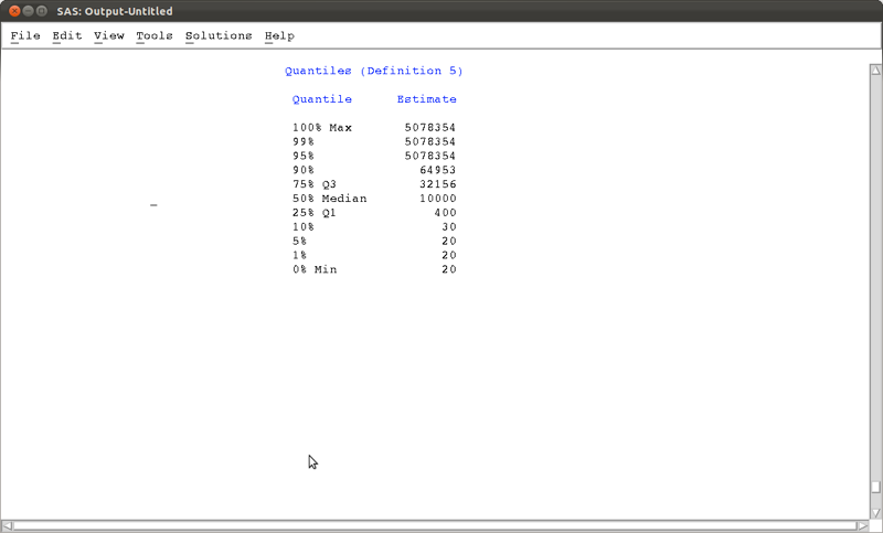
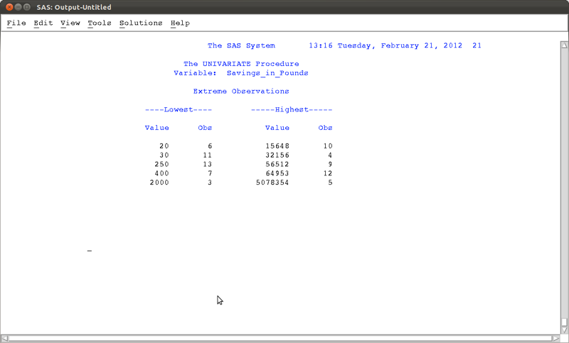
proc univariate data=mat013.mmm;
var savings_in_pounds;
run;
The various outputs of the "univariate" procedure are shown.
### Frequency tables
The "freq" procedure allows us to obtain frequency tables of data sets. As an example, let's consider the dataset shown.
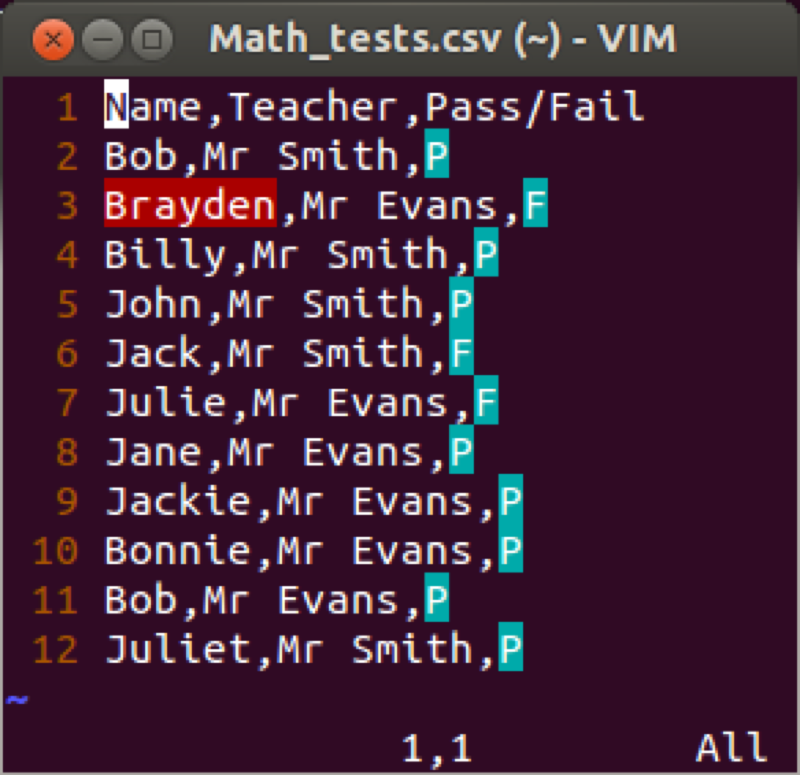
The most basic "freq" procedure will give the frequencies of all the observations in the data set:
proc freq data=mat013.math_tests;
run;
We can specify the variables we want to look at by listing them after the "tables" statement (similar to the var statement for the "means" procedure):
proc freq data=mat013.math_tests;
tables teacher pass_fail;
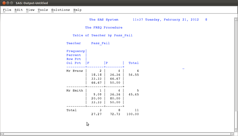
run;If we want to cross tabulate the data then we use a * in between the variables concerned:
proc freq data=mat013.math_tests;
tables teacher*pass_fail;
run;
The above code gives the table shown.
Various options can be passed to the "freq" procedure, the simplest of which is shown below:
proc freq data=mat013.math_tests;
tables teacher*pass_fail / nocol norow nopercent;
run;
Other options include computing a chi square test but we will not worry about that for now.
2.2.2 Correlations
The "corr" procedure can be used to obtain correlations in SAS. The following code is the basic "corr" procedure applied to the mat013.mmm data set which gives the output shown.
proc corr data=mat013.mmm;
run;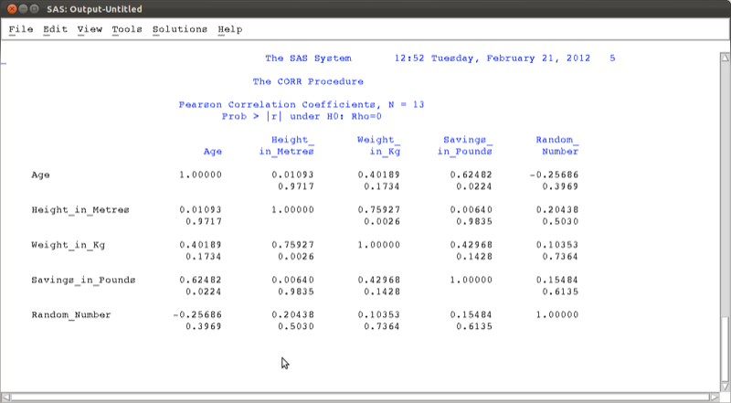
If we want to run the "corr" procedure on a subset of the variables then we use the "var" statement:
proc corr data=mat013.mmm;
var age savings_in_pounds;
run;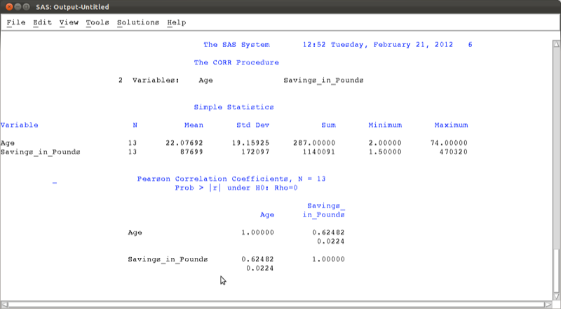
2.2.3 Linear Models
In this section we'll very briefly see the syntax for some basic linear models in SAS. First of all we'll take a look at linear regression. The following code will run such an analysis on the mat013.jjj data set, checking if there is a linear model of height with predictors weight and savings:
proc reg data=mat013.jjj;
model height_in_metres=weight_in_kg savings_in_pounds;
run;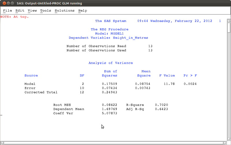
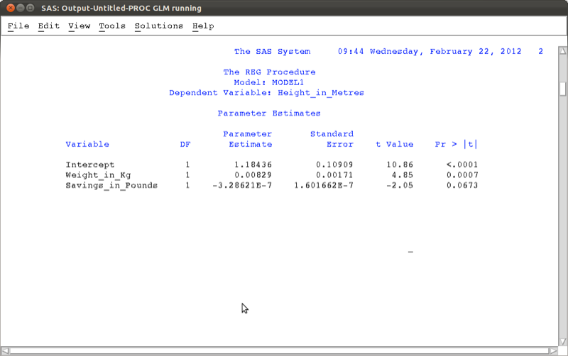
Looking at the p-value we see that the overall model should not be rejected, however the detailed results show that perhaps we could remove savings from the model.
Analysis of variance (ANOVA) can be done very easily in SAS. We show this using a new data set.
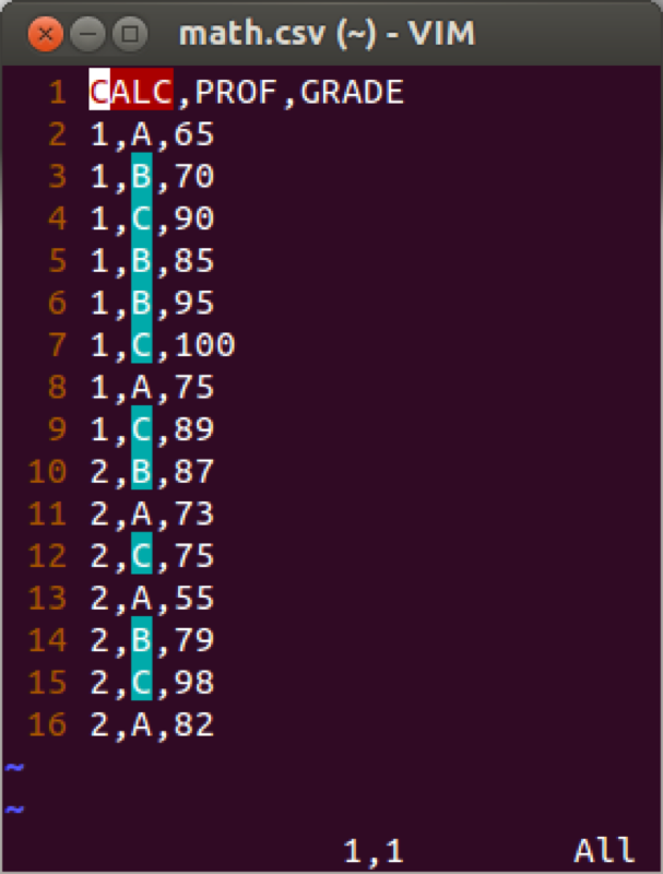
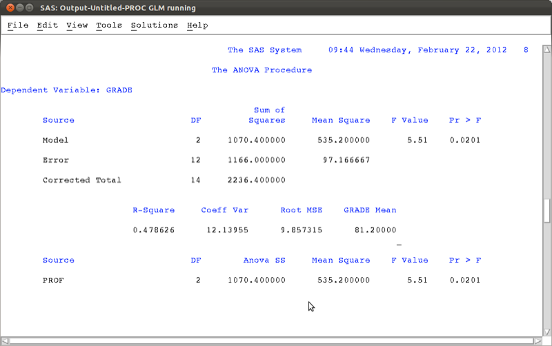
We will use the "anova" procedure to see if the grades obtained by students depend on their teacher.
proc anova data=mat013.math;
class prof;
model grade=prof;
run;
Note the "class" keyword is needed to state which variable we are using to group on. The results show that there is indeed a difference between groups (further post-hoc tests are needed to investigate which groups differ etc.).
Another procedure that can be used for a variety of models (including the 2-way anova) is the "glm" (general linear model) procedure. The following code simply reproduces the above results.
proc glm data=mat013.jjj;
model height_in_metres=weight_in_kg savings_in_pounds;
run;

proc glm data=mat013.math;
class prof;
model grade=prof;
run;
2.2.4 Plots and charts
There are various ways to obtain histograms in SAS, the easiest way is to use the "univariate" procedure with the "histogram" option. The following code gives a histogram for the height of individuals in the mat013.jjj dataset as shown.
proc univariate data=mat013.jjj;
var height_in_metres;
histogram;
run;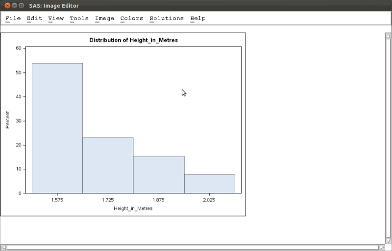
There are various ways to obtain scatter plots in SAS, the easiest way is to use the "gplot" procedure. The following code gives a scatter plot for the height of individuals against their weight in the mat013.jjj dataset as shown.
proc gplot data=mat013.jjj;
plot height_in_metres*weight_in_kg;
run;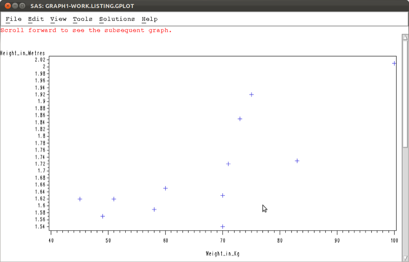
There are various other ways to obtain similar graphs as well as change the look and feel of our graphs. We won't go into this here but you are encouraged to look into it.
2.3 Exporting output
We can output results of procedures in SAS using the "output delivery system". The syntax is straightforward and we surround normal SAS code with the "ods" statements to output to various formats (html, pdf, rtf).
ods [format of your choice] file=[Location of file to be output];
[Normal SAS code]
ods [format of your choice] close;
As an example, the following code creates an html file called "freq_table" in html format stored at the location "~/Desktop" (note that in Window's the / should be a \) as shown.
ods html file="\~/Desktop/freq_table.htm";

proc gplot data=mat013.jjj;
plot height_in_metres*weight_in_kg;
run;

ods html close;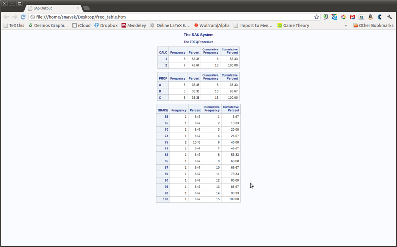
The following code will create a file called "scatter_plot.pdf" in pdf format stored at the location "~/Desktop" (note that in Window's the "/" should be a "") as shown.
ods pdf file="\~/Desktop/scatter_plot.pdf";

proc gplot data=mat013.jjj;
plot height_in_metres*weight_in_kg;
run;

ods pdf close;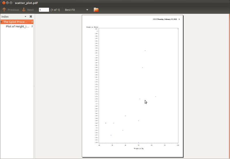
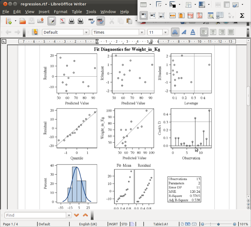
The following code will create a file called "regression.rtf" in rtf format (Word, LibreOffice etc.) stored at the location "~/Desktop" (note that in Window's the "/" should be a "") as shown.
ods rtf file="\~/Desktop/regression.rtf";

proc reg data=mat013.jjj;
model weight_in_kg=height_in_metres;
run;

ods rtf close;