R Chapter 5 - Further packages
In this chapter we will examine three packages in particular:
- sqldf: a package allowing for the use of sql syntax in R
- ggplot2: a powerful package for the plotting of data
- twitteR: a package that allows for the data mining of twitter
5.1 sqldf
5.1.1 Basic SQL
SQL is a language designed for querying and modifying databases. Used by a variety of database management software suites:
- Oracle
- Microsoft ACCESS
- SPSS
SQL uses one or more objects called TABLES where: rows contain records (observations) and columns contain variables.
To use SQL in R we need to use the sqldf package.
The following code creates a data set called test in the work library as a copy of the mmm data set:
test<-sqldf("select * from MMM")The "*" command tells R to take all variables from the data set. We can however specify exactly what variables we want:
test<-sqldf("select Name,Age,Sex from MMM")We can also create new variables:
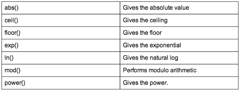
test<-sqldf("select Name,Age,Sex,Weight_in_Kg/(power(Height_in_Metres,2)) as bmi from MMM")Some of the SQL operators are shown.
5.1.2 Further sql
In this section we'll take a look at what else R can do with sql. For the purpose of the following examples let's write a new data set:
Var1<-c("A","A","B","C","C")
Var2<-c(1,1,1,2,2)
Var3<-c("A","A","A","B","C")
Var4<-c(2,2,1,2,1)
Var5<-c("B","B","C","D","E")

example<-data.frame(Var1,Var2,Var3,Var4,Var5)
Some simple SQL code very easily helps us to get rid of duplicate rows (this can be very helpful when handling real data). To do this we use the "distinct" keyword.
sqldf("select distinct * from example")We can also select particular variables:
sqldf("select distinct Var1,Var2,Var3 from example")We can also use the "where" statement to select variables that obey a particular condition:
sqldf("select * from example where Var2<=Var4")We can sort data sets using the "order by" keyword:
sqldf("select distinct * from example order by Var1")A very nice application of SQL is in the aggregation of summary statistics. The following code creates a new variable that gives the average value of var2. The value of this variable is the same for all the observations:
sqldf("select avg(Var2) as average_of_Var2 from example")We could however get something a bit more useful by aggregating the data using a "group" statement:
sqldf("select Var1,avg(Var2) as average_of_Var2 from example group by Var1")
5.1.3 Joining tables with SQL
A very common use of SQL is to carry out "joins" which are equivalent to a merger of data sets. There are 4 types of joins to consider:
inner join
- output table only contains rows common to all tables
- variable attributes taken from left most table
outer join left
- output table contains all rows contributed by the left table
- variable attributes taken from left most table
outer join right
- output table contains all rows contributed by the right table
- variable attributes taken from right most table
outer join full
- output table contains all rows contributed by all tables
- variable attributes taken from left most table
To work with these examples let's use the data sets created with the following code:
Owner<-c("Jeff","Janet","Paul","Joanna")
Name<-c("Ruffus","Sam",NA,NA)
Dogs<-data.frame(Owner,Name)

Owner<-c("Jeff","Paul","Joanna","Vince")
Name<-c("Kitty",NA,"Tinkerbell","Chick")
Cats<-data.frame(Owner,Name)
The following code carries out an inner join of these two datasets also changing the name of the "Name" variable depending on which data set it was from.
sqldf("select a.Owner, a.Name as Dog_Name, b.Name as Cat_Name from Dogs as a, Cats as b where a.Owner=b.Owner")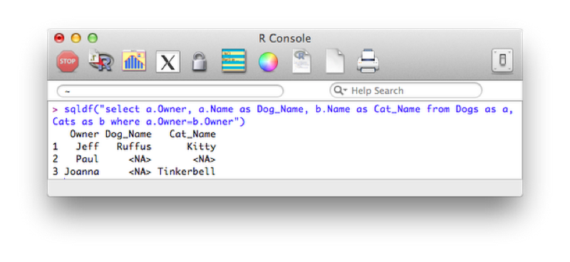
The following code carries out a left outer join, the output of which is show.
sqldf("select a.Owner, a.Name as Dog_Name, b.Name as Cat_Name from Dogs as a left join Cats as b on a.Owner=b.Owner")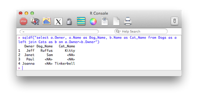
Right and full outer joins are not yet supported in sqldf however they can actually be obtained by simply using the "merge" function (as discussed in Chapter 3).
5.2 ggplot2
This is an extremely powerful package that allows for the creation of publication quality plots with ease. There are two basic functions in ggplot2:
- qplot which allows us obtain quick graphs
- ggplot which gives us more control of granularity (we will not go into it here)
5.2.1 Basic plots with qplot
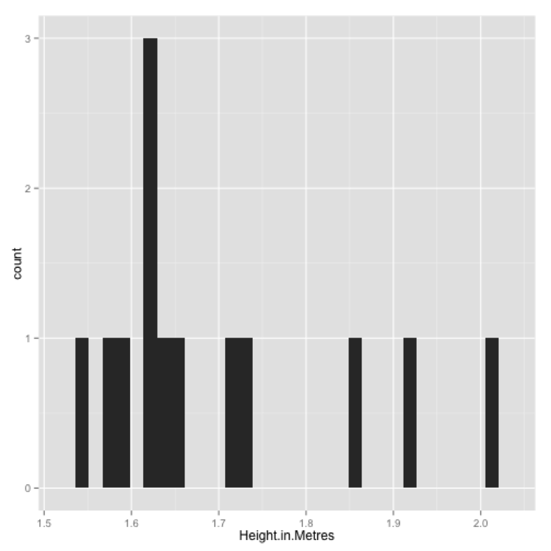
The qplot command is very similar to the plot command in that in will often produce the plot required based on the inputs. To obtain a histogram of the Height.in.Metres variable of the JJJ data set we simply use:
qplot(data=JJJ,x=Height.in.Metres)This produces the plot shown.
We can improve this by changing the bin width, including a title and changing the labels for the x axis and y axis.
qplot(data=JJJ,x=Height.in.Metres,binwidth=.075,main="Height of people in the JJJ data set",xlab="Height",ylab="Frequency")
We can obtain a density plot corresponding to the above by using the "density" option for the "geom" argument as shown:
qplot(data=JJJ,x=Height.in.Metres,binwidth=.075,main="Height of people in the JJJ data set",xlab="Height",ylab="Frequency",geom="density")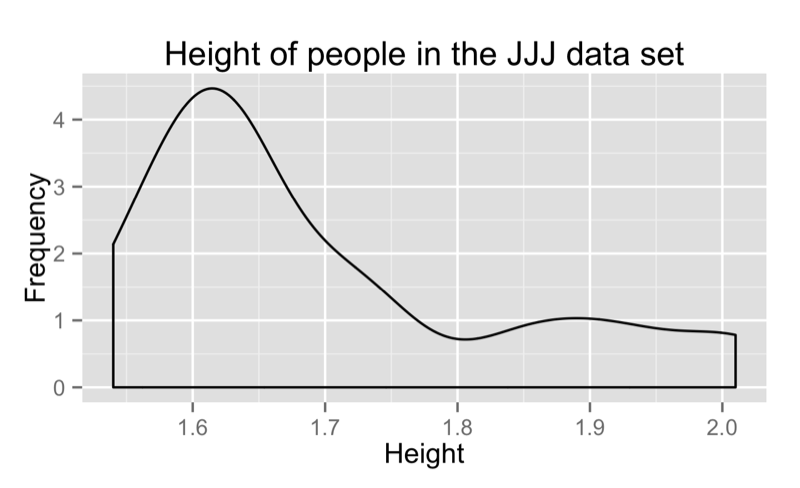
If we pass two vectors to qplot we obtain a scatter plot:
qplot(data=JJJ,x=Weight.in.Kg,y=Height.in.Metres)we can also pass qplot a "size" argument to obtain the graph shown:
qplot(data=JJJ,x=Height.in.Metres,y=Weight.in.Kg,size = Age)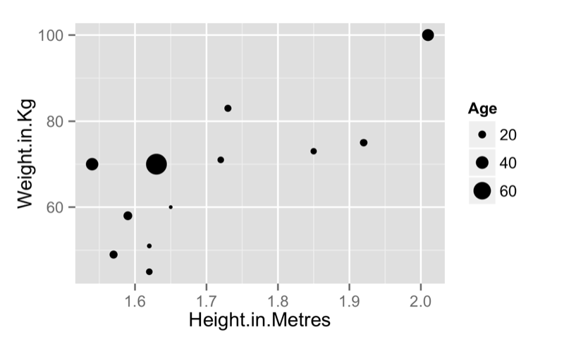
We can of course obtain scatter plots against categorical variables as shown:
qplot(data=JJJ,x=Sex,y=Height.in.Metres)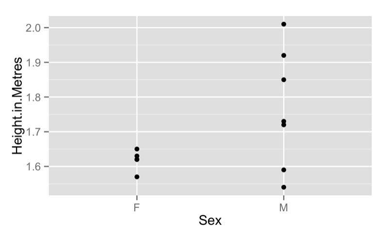
We can pass "boxplot" as the "geom" argument to get a boxplot as shown.
qplot(data=JJJ,x=Sex,y=Height.in.Metres,geom='boxplot')
5.2.2 Advanced features
We can add various features to our scatter plot. The following code just plots a line between all the points:
qplot(data=JJJ,x=Height.in.Metres,y=Weight.in.Kg,geom="line")We can combine various geom options so as to not just include a line but also the points:
qplot(data=JJJ,x=Height.in.Metres,y=Weight.in.Kg,geom=c("point","line"))Finally we can also add a smoothed line to our plot as shown:
qplot(data=JJJ,x=Height.in.Metres,y=Weight.in.Kg,geom=c("point","line","smooth"))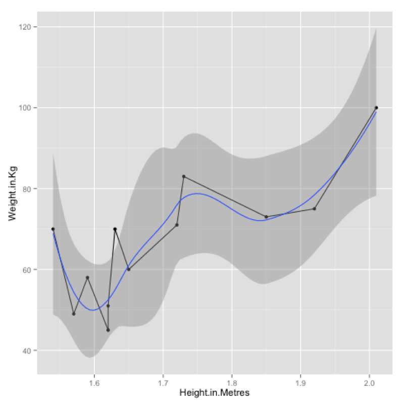
We can very easily obtain a collection of any of the above plots across a categorical variables using the "facets" command as shown:
qplot(data=JJJ,x=Height.in.Metres,binwidth=.075,facets=~Sex)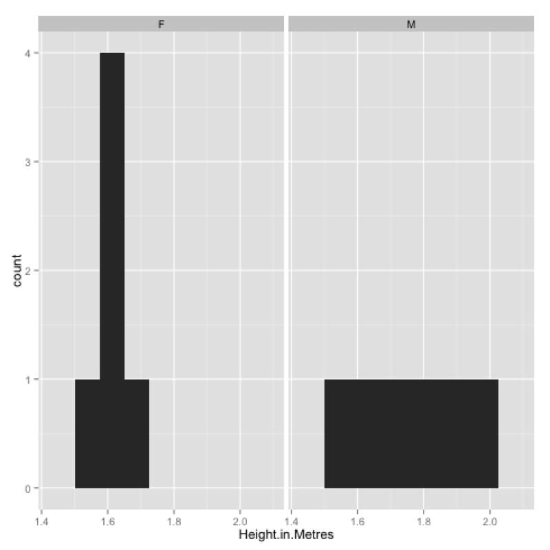
We can use the "ggsave" command to save the last plotted graph to file:
ggsave(filename="~/Desktop/test.pdf")One final aspect we will take a look at in ggplot2 is that of layers. To do so we will use the following dataset:
MMMJJJ_to_plot<-within(MMMJJJ,{data_set<-ifelse(substr(MMMJJJ$Name,1,1)=="M","MMM","JJJ");Sex<-substr(Sex,1,1)})Firstly we create a plot using qplot and assign it to p (recall that everything in R is an object).
p<-qplot(data=MMMJJJ_to_plot,x=Height.in.Metres,y=Weight.in.Kg,facets=~data_set~Sex,color=Sex)To view the plot we simply type "p" (note that we have also included a "color" option):
pFinally we can add a new layer to this plot by "adding" (+) a linear model to our graph:
p<-p+stat_smooth(method="lm")The output of all this is shown.
Finally we can save a particular graph object in ggplot using ggsave:
ggsave(p,filename="~/Desktop/plot.pdf")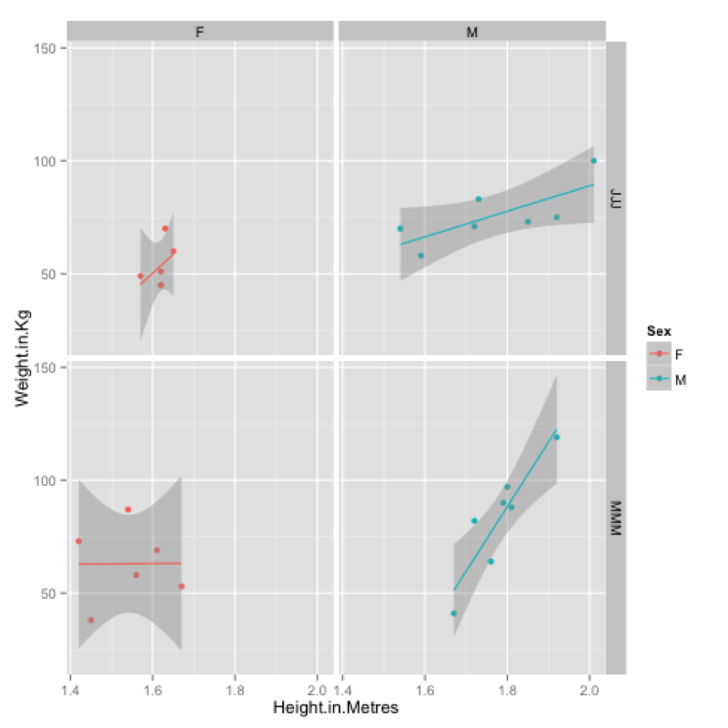
5.3 twitteR
The last package we will consider is a package that can be used to data mine twitter.
To get the certain trends we use can use the following code:
getTrends(period = "daily", date=Sys.Date())
getTrends(period = "daily", date=Sys.Date() - 1)
getTrends(period = "weekly")
To obtain tweets for a particular hashtag:
searchTwitter("#orms")Finally to obtain tweets from a particular user (the following gives the tweets of the INFORMS as shown):
userTimeline("INFORMS")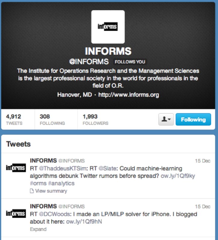

(Other versions of the above: pdf docx (not recommended))