R Chapter 4 - Programming
4.1 Flow Control
A huge part of programming (in any language) is the use of so called "conditional statements" that allow for flow control. We do this in R using "if" statements.
There are two types of "if" statements in R. The simple "if" statement as shown below:
x<-39
if (x>20) y<-1
We can use this in conjunction with an "else" statement:
x<-19
if (x>20) y<-1 else y<-0
Finally, the if-else call is a function and as such we can rewrite the above code as:
y<- if (x>20) 1 else 0Finally we can include multiple commands as outcomes of an if statement by using "{}":
x<-20
if (x==21) {
y<-1
z<-"T"
} else{
y<-0
z<-"F"}
The above statements checks a single value and whilst we'll learn in the next section how to loop offer sets of values it is very much worth learning how to use the 'vectorized' form of the if statement: the "ifelse" command. The general syntax is given below:
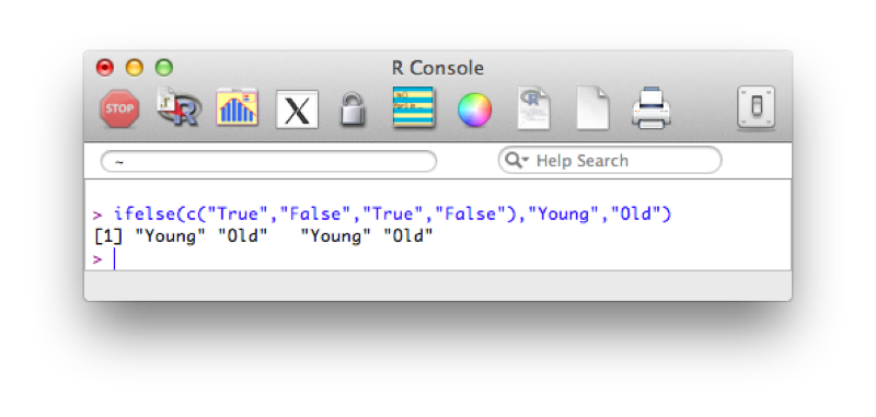
ifelse(Boolean_Vector,Outcome_If_True,Outcome_If_False)An example of this is given below:
ifelse(c("True","False","True","False"),"Young","Old")The output is shown.
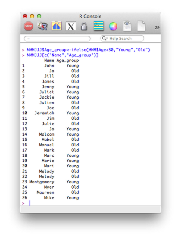
Using this and our knowledge of filtering we see how we can create new variables using the ifelse statement. The following code creates a new variable "age_group":
MMMJJJ$Age_group<-ifelse(MMM$Age<30,"Young","Old")
MMMJJJ[c("Name","Age_group")]
The output is shown.
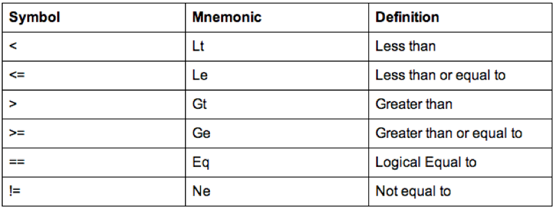
Some of the comparison operators that can be used in conjunction with 'if' statements are shown.
A further important notion in programming is the notion of loops. There are two types of loops that we will consider:
- for
- while
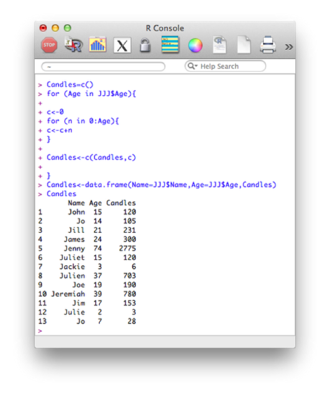
The for loop allows us to compute iterative procedures. As with most things in R, the for loop iterates a value over a vector. The following code outputs the total number of birthday candles that would have been used on everyones birthday cake in the JJJ data set.
Candles=c()
for (Age in JJJ$Age){
c<-0
for (n in 0:Age){
c<-c+n
}
Candles<-c(Candles,c)
}
Candles<-data.frame(Name=JJJ$Name,Age=JJJ$Age,Candles)
The first statement creates an empty vector called "Candles". The first for loop, loops over the age variable in the JJJ data set ("0:age" is in fact a short way of writing a vector of integers from 0 to age). For each of those values of age we use a second for loop to sum the total number of candles and concatenate that value to the vector Candles. Finally we create a new data set Candles by concatenating the various vectors required (note that we're also renaming certain variables here).
Note that in general this is not the most efficient way of undertaking things in R. Vectorized versions of the above are much faster (we won't cover these here). Another improvement for the above code is to create the vector Candles initially as a vector of the correct size and type. For example we can create a numeric vector of a certain length using the following code (all initial values will be set to 0):
Candles=vector("numeric",length=length(JJJ$Age))Using this the above code would be written as:
Candles=vector("numeric",length=length(JJJ$Age))
k<-0
for (Age in JJJ$Age){
k<-k+1
c<-0
for (n in 0:Age){
c<-c+n
}
Candles[k]<-c
}
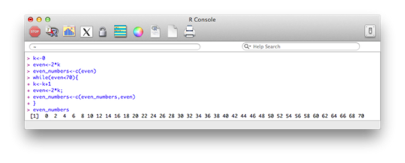
Candles<-data.frame(Name=JJJ$Name,Age=JJJ$Age,Candles)The second type of loop we will consider is the do while loop. This loop checks a condition before carrying out an operation. The following code creates a vector with all even numbers less than 70:
k<-0
even<-2*k
even_numbers<-c(even)
while(even<70){
k<-k+1
even<-2*k;
even_numbers<-c(even_numbers,even)
}
The output is shown.
4.2 Functions
One of the great capacities of R is the ease with which one can create new functions. The general syntax for this is given by:
myfunction <- function(arg1, arg2, ... ){
statements
return(object)
}
The return statement is very important as it indicates the "result" of the function. This can be any R object, a vector, a data frame etc... Note that is can also be omitted, as long as the last command is what you want returned.
The following code creates a function called "f1" that adds 3 to a number if it is even and adds 2 to a number if it is odd.
f1 <- function(x){
r <- if (x%%2==0) x+3 else x+2
return(r)
}
To run the function we would then use it like any other R function. For example the following would return 11.
f1(9)(The %% command return the modulo of the first number with respect to the second)
We can also create a function with no arguments that simply replicates shorthand for some code:
My_plot <- function(){
r<-hist(JJJ$Height.in.Metres)
return(r)
}

My_plot()
The following code defines a function that creates a new dataset entitled "JJJ_after_shopping" that subtracts a quantity from the savings variable in the JJJ dataset:
shopping <- function(spend){
New.Savings<-JJJ$Savings.in.Pounds-spend
JJJ_after_shopping<-data.frame(JJJ$Name,Old.Savings=JJJ$Savings.in.Pounds,New.Savings)
return(JJJ_after_shopping)
}
Note that this function makes use of recycling (when creating the New.Savings vector).

We can of course define functions with multiple arguments as below:
shopping <- function(spend,trips){
New.Savings<-JJJ$Savings.in.Pounds-trips*spend
JJJ_after_shopping<-data.frame(JJJ$Name,Old.Savings=JJJ$Savings.in.Pounds,New.Savings)
return(JJJ_after_shopping)
}
It's also possible to set certain values as defaults:
shopping <- function(spend,trips=1){
New.Savings<-JJJ$Savings.in.Pounds-trips*spend
JJJ_after_shopping<-data.frame(JJJ$Name,Old.Savings=JJJ$Savings.in.Pounds,New.Savings)
return(JJJ_after_shopping)
}
4.3 Vectorising
In general the for loops we have seen can be written in a much more efficient way using function and various forms of the apply function (which apply functions over vectors, lists and matrices):
- apply
- lapply
- sapply
- mapply
Note that an array in R is a very generic data type; it is a general structure of up to eight dimensions. For specific dimensions there are special names for the structures. A zero dimensional array is a scalar or a point; a one dimensional array is a vector; and a two dimensional array is a matrix. The general syntax of the apply function is given below:
apply(matrix,margin,function)We have not yet seen matrices but they are relatively simple to understand: 2 dimensional objects. The following code produces a 2 by 3 matrix:
mat<-matrix(c(1,2,3,4,5,6),2,3)
mat
The "margin" option (either 1,2 or both (1:2)) simply tells R what dimension to apply the required function to, experiment with the following:
apply(mat,1,mean)
apply(mat,2,mean)
apply(mat,1:2,mean)
We can use the apply function on data frames and vectors but in general it will be easier to use the "lapply" function which simply applies a function to a 1 dimensional object. The lapply function becomes especially useful when dealing with data frames. In R the data frame is considered a list and the variables in the data frame are the elements of the list. We can therefore apply a function to all the variables in a data frame by using the lapply function. Note that unlike in the apply function there is no margin argument since we are just applying the function to each component of the list. The following code simply returns the sqaure roots of a vector.
lapply(c(1,2,3,4,5),sqrt)Note that the above returns a list (an R object that we will not pay much attention to here). We can get a vector by using the following:
unlist(lapply(c(1,2,3,4,5),sqrt))The "sapply" function is simply a version of lapply that by default returns the most appropriate object type. The following code gives the exact same result as above:
sapply(c(1,2,3,4,5),sqrt)Finally, there exists a multivariate example of the above function which allows us to pass multiple arguments to a function. The following code defines a simple function:
simple_function<-function(x,y) x/yWe can now apply this function so that it takes the consecutive ratios of two vectors:
mapply(simple_function,1:4,4:1)With these functions we can drastically improve the performance of R code. The following reproduces code from before:
my_sum<-function(x){
sum(x)
}

sapply(JJJ$Age,my_sum(1:x))
Note that there is no need to actually define the function we can refer directly to the function object:
sapply(JJJ$Age,function(x) sum(1:x))4.4 Handling strings
SAS is a macro language and philosophically macros allow a user to substitute pieces of text for a variable, and evaluate the result. R is not a macro language and thus does the opposite: evaluates the arguments and then uses the values.
The paste command allows us to concatenate strings. The following code outputs the string "Hello-World". Note that we can use any string as a separator (include the empty string "").
x<-"Hello"
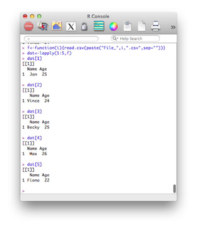
paste(x,"World",sep="-")This immediately allows for quite complex manipulation of data files. For example the following code, imports the 5 datafiles File_1.csv - File_5.csv:
f<-function(i){read.csv(paste("File_",i,".csv",sep=""))}
dat<-lapply(1:5,f)
Note that this piece of code introduces a new structure a bit more formally. The object "dat" is here a list and we use the "lappy" function (we haven't seen this yet) to apply the newly created function "f" (that imports data).
The output is shown.
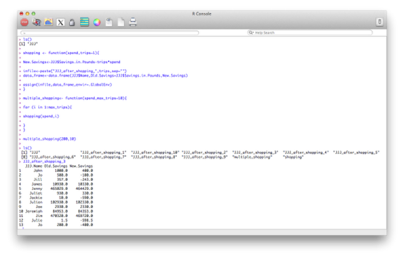
We can also revisit a previous function (the shopping function) and create a different data set for every value of spend. We'll even make this a bit more complicated and nest functions so that we can repeat this operation for various values of the variable "spend".
shopping <- function(spend,trips=1){
New.Savings<-JJJ$Savings.in.Pounds-trips*spend
infile<-paste("JJJ_after_shopping_",trips,sep="")
data_frame<-data.frame(JJJ$Name,Old.Savings=JJJ$Savings.in.Pounds,New.Savings)
assign(infile,data_frame,envir=.GlobalEnv)
}

multiple_shopping<- function(spend,max_trips=10){

for (i in 1:max_trips){
shopping(spend,i)
}
}
Note the extra option that has been passed to the "assign" command "envir=.GlobalEnv". This is to ensure that the data sets created in the function are global (i.e. are still there when the function stops running).
4.5 Memory and scripts.
In this section we will take a brief look at how R handles the "workspace". If you have already quit R you would have seen the prompt "Save workspace image?". If you answer "yes" then R saves various things to various files (in the current working directory): 1. .Rdata holds all the objects (data frames, vectors, functions etc...) currently in memory (note that this file is written in an R specific file and so can't be read). 2. .Rhistory holds all the commands used (and so can be recalled).
Being prompted whether or not to save the workspace is helpful (in my opinion) as you can simply open an R session to try a few things and not save (similar to using the work library in SAS). It is possible to save the workspace image as you go (this is worthwhile in case your system happens to crash):
save.image()Note: we can leave the argument of the "image" function empty (as above), in which case the file will be saved in the current directory. We can also pass the required location to the "image" function.
It is also possible to save particular objects to particular files as well as load files but we won't go into that here.
One final aspect to consider is that of running script files from the command line. We do this using the "source" command. Note that this command executes all the code in the script as if it was typed in one after the other. To see this let us write the following code in a text file (saving it as "first_script.r" on the desktop for example):
x<-c(1,2,3,4)
y<-c(1,0)
print(x+y)
print(x*y)
We then run the script using the following code:
source("~/Desktop/first_script.r")Repetitive command that are run often (for example, routine data analysis) can be saved as scripts and called if and when new data is received.